9 The Derivative
9.1 From Linear Maps to Differentiation
We have developed the theory of vectors, linear maps, and functionals. We now use this machinery to define the derivative.
9.1.1 Local Linearity
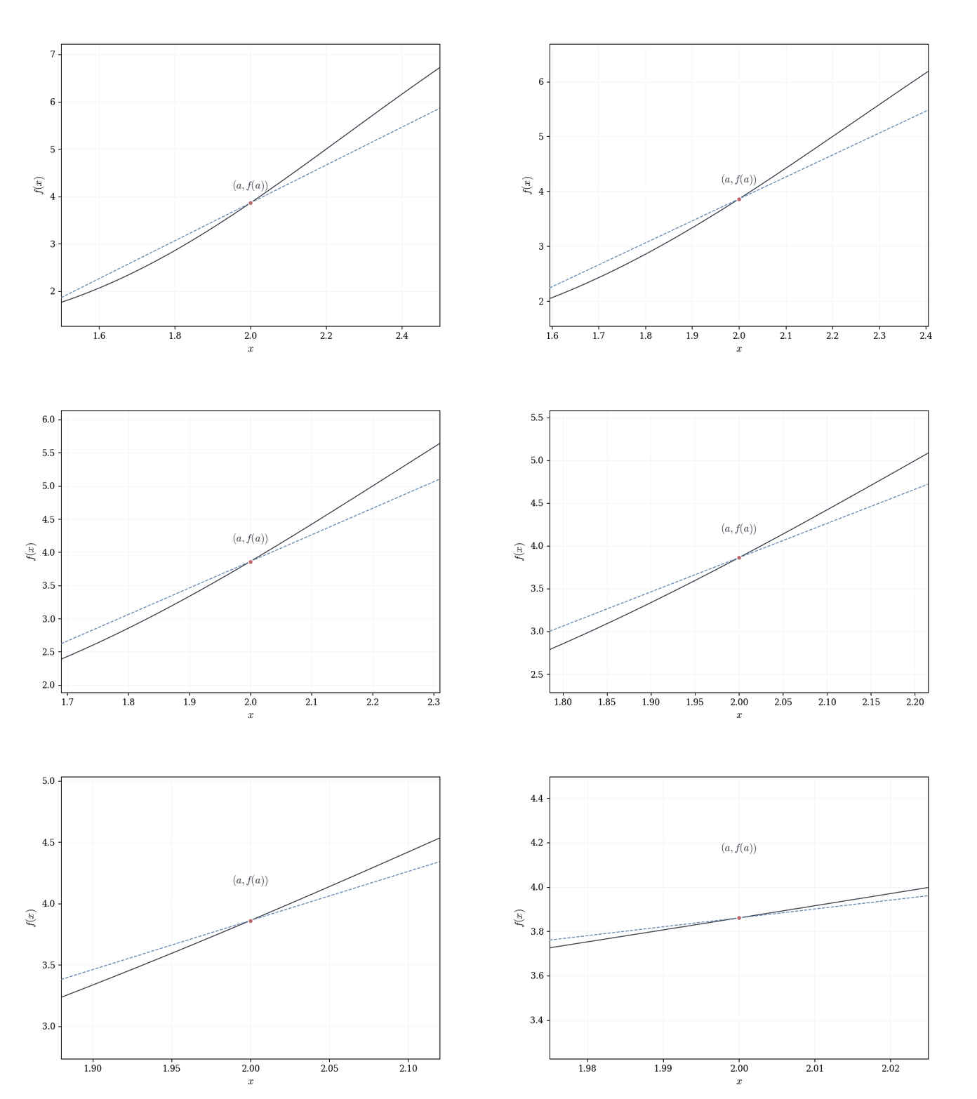
Let f : \mathbb{R} \to \mathbb{R} be smooth, and fix a \in \mathbb{R}. The graph of f near (a, f(a)) appears approximately linear.

This suggests the following question: can one associate to f at a a linear map that approximates the change in f near a?
9.1.2 Linear Approximations
To approximate f near a, one might consider a constant function: f(a+h) \approx f(a). This neglects the rate of change of f at a. A quadratic approximation, f(a+h) \approx f(a) + b h + c h^2, captures curvature, but requires two parameters. For the purpose of measuring instantaneous change, a linear approximation suffices:
f(a+h) \approx f(a) + m h,
where m is a scalar. The predicted change is proportional to the displacement: doubling h doubles the predicted change, and reversing h reverses it.
9.1.3 Linear Maps and Differentials
Recall that a map T : \mathbb{R} \to \mathbb{R} is linear if
T(x+y) = T(x) + T(y), \quad T(\lambda x) = \lambda T(x) \quad \forall x,y \in \mathbb{R}, \lambda \in \mathbb{R}.
Every such map has the form T(h) = mh for some m \in \mathbb{R}. Linear functionals are linear maps into \mathbb{R}; they assign a scalar to each input vector. The differential of f at a is such a functional:
df_a(h) \approx f(a+h) - f(a).
Since df_a is linear, there exists m \in \mathbb{R} such that
df_a(h) = m h.
This scalar m is called the derivative of f at a, denoted f'(a).
df_a denotes the linear map \mathbb{R} \to \mathbb{R}.
f'(a) denotes its coordinate representation.
Relation: df_a(h) = f'(a) \cdot h.
In higher dimensions, f'(a) becomes the Jacobian matrix; the framework remains unchanged.
9.1.4 Measuring the Quality of Approximation
Let T(h) = m h. Define the error
E(h) = f(a+h) - f(a) - T(h).
Absolute error alone is insufficient. One considers the normalized error |E(h)|/|h|. A linear map T is a first-order approximation of f at a if
\lim_{h \to 0} \frac{|f(a+h) - f(a) - T(h)|}{|h|} = 0.
In this case, T captures the first-order behavior of f at a, and df_a is called the differential of f at a.
9.1.5 A Concrete Example
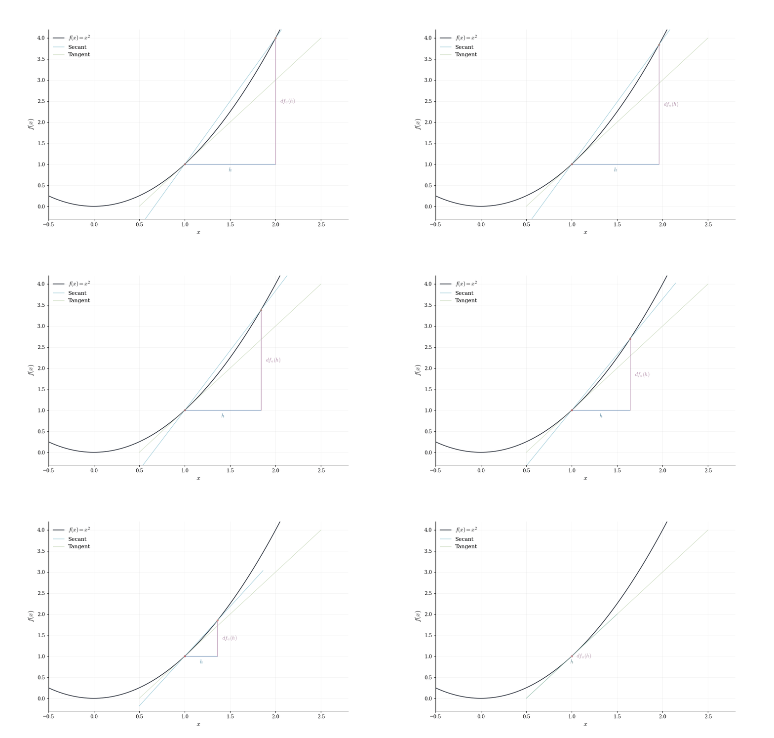
Let f(x) = x^2 and consider the point a = 1. For a small displacement h, direct computation gives f(1+h) = (1+h)^2 = 1 + 2h + h^2.
We identify the linear term 2h and the error E(h) = h^2. Is this error negligible relative to h? We compute \frac{|E(h)|}{|h|} = \frac{|h^2|}{|h|} = |h| \to 0 \quad \text{as } h \to 0.
Indeed, the linear map T(h) = 2h approximates the change in f near a = 1 with vanishing relative error. The coefficient 2 is the derivative f'(1) = 2.

The general pattern: expand f(a+h), identify the linear term, verify that the remainder is o(h), and recognize the coefficient of the linear term as the derivative.
9.2 The Formal Definition
Definition 9.1 (Differentiability) Let f : I \to \mathbb{R} where I is an interval, and let a be an interior point of I. We say f is differentiable at a if there exists a linear map T : \mathbb{R} \to \mathbb{R} such that \lim_{h \to 0} \frac{|f(a+h) - f(a) - T(h)|}{|h|} = 0.
Since every linear map in one dimension has the form T(h) = m h, we write T(h) = f'(a) h, and the scalar f'(a) is called the derivative of f at a.
9.2.1 Alternative formulation
Dividing the approximation error by h and rearranging,
\frac{f(a+h) - f(a)}{h} = f'(a) + \frac{E(h)}{h}.
As h \to 0, the right side approaches f'(a). Thus differentiability is equivalent to the existence of the limit f'(a) = \lim_{h \to 0} \frac{f(a+h) - f(a)}{h}.
This is the classical difference quotient definition. Both formulations are equivalent, but the linear map perspective emphasizes that the derivative is fundamentally about approximation by a linear transformation.
Notation: We write f'(a), \frac{df}{dx}\big|_{x=a}, or Df(a) for the derivative at a. The notation Df(a) emphasizes the derivative as a linear map, a viewpoint essential in higher dimensions.
If a function is well-approximated by a linear map near a point, what does this tell us about the function’s behavior at that point? Linear maps are continuous—they can’t have jumps or breaks. If f is close to a linear map near a, it seems reasonable that f itself should be continuous at a. This intuition is correct and leads to one of the most important basic facts about derivatives.
Theorem 9.1 (Differentiability Implies Continuity.) Let f : I \to \mathbb{R} and a \in I. If f is differentiable at a, then f is continuous at a.
Differentiability means there exists a linear map T(h) = f'(a) h such that f(a+h) = f(a) + T(h) + o(h), \quad h \to 0.
By definition of o(h), for any \varepsilon > 0 there exists \delta > 0 such that |h| < \delta implies \frac{|f(a+h) - f(a) - f'(a) h|}{|h|} < \varepsilon.
Hence |f(a+h) - f(a)| = |f'(a) h + o(h)| \le |f'(a)|\,|h| + |o(h)| < (|f'(a)| + \varepsilon) |h|.
As h \to 0, the right-hand side tends to 0. Therefore, \lim_{h \to 0} f(a+h) = f(a), so f is continuous at a. \square
9.3 Linear Approximation and the Tangent Line
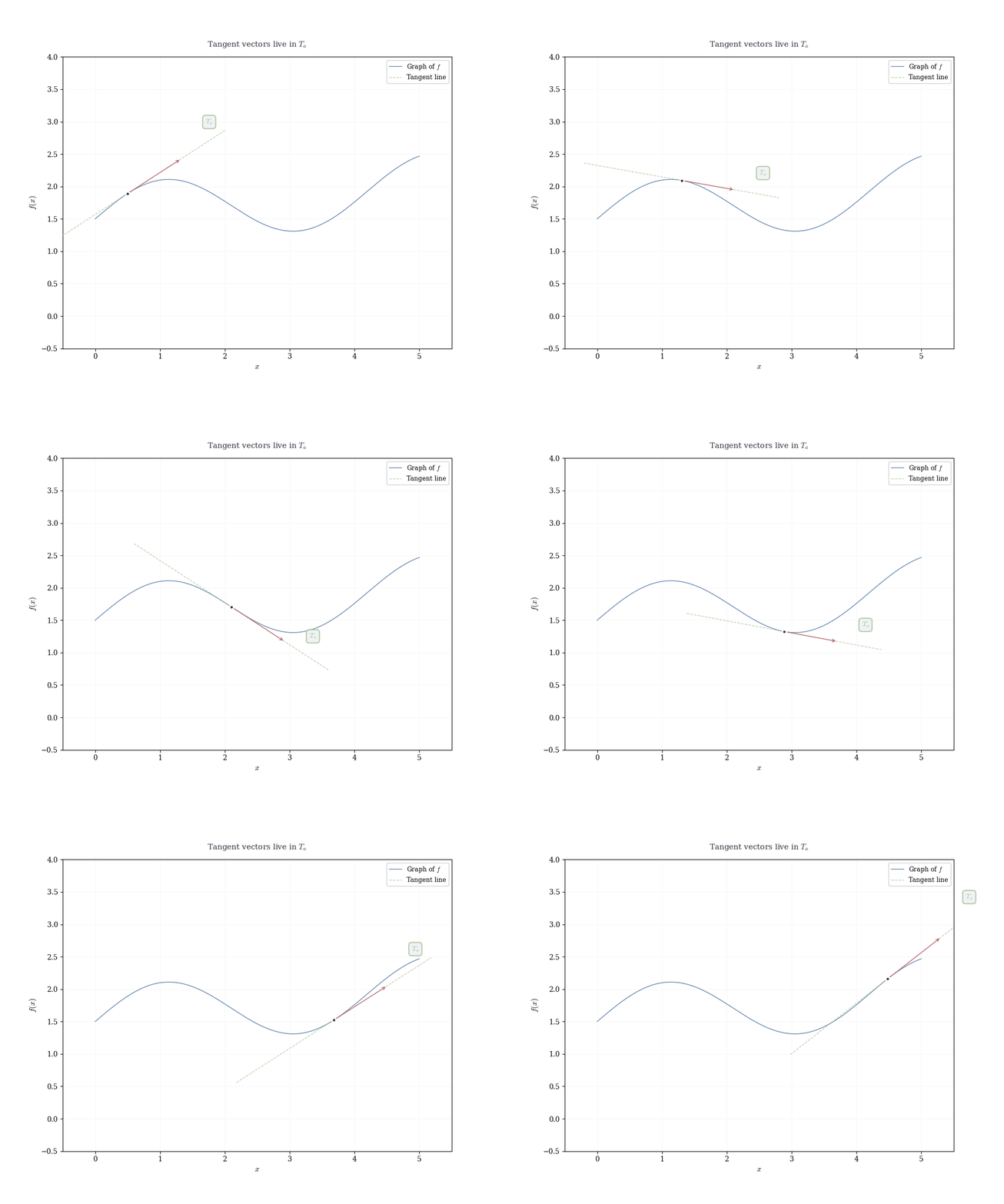
If f is differentiable at a, the linear map df_a(h) = f'(a) h determines the tangent line to the graph of f at (a, f(a)).

Recall that a linear map in 1D is completely determined by where it sends the basis vector 1: df_a(1) = f'(a) \cdot 1 = f'(a).
This single value encodes the entire linear transformation. Geometrically, it’s the slope of the tangent line. Algebraically, it’s the functional that measures change.
Writing x = a + h, the linear approximation becomes f(x) \approx f(a) + f'(a)(x - a), which is the equation of the tangent line.
Near x = a, the function f(x) is well approximated by this linear function. The derivative f'(a) is the slope of the tangent line, but more fundamentally, it is the coefficient of the linear map that best approximates the change in f near a.
9.4 The Differential and Linear Functionals
The differential df_a is a linear functional in the sense of Section 8.5. It takes a displacement h \in \mathbb{R} and returns a scalar df_a(h) = f'(a)h \in \mathbb{R}.
In coordinates, if we think of h as the column vector \begin{pmatrix} h \end{pmatrix} and f'(a) as the row vector \begin{pmatrix} f'(a) \end{pmatrix}, then df_a(h) = \begin{pmatrix} f'(a) \end{pmatrix} \begin{pmatrix} h \end{pmatrix} = f'(a) \cdot h.
In one dimension, the distinction between f'(a) (a scalar) and df_a (a linear functional) is subtle: they contain the same information. The functional df_a is simply multiplication by the scalar f'(a).

9.4.0.1 Examples
Example 9.1 (Derivative of x^2) Let f(x) = x^2 and compute f'(a).
We seek a linear map T(h) = mh such that \lim_{h \to 0} \frac{|(a+h)^2 - a^2 - mh|}{|h|} = 0.
Expanding (a+h)^2 = a^2 + 2ah + h^2, we have \frac{|a^2 + 2ah + h^2 - a^2 - mh|}{|h|} = \frac{|(2a - m)h + h^2|}{|h|} \leq |2a - m| + |h|.
This approaches zero as h \to 0 if and only if m = 2a. Thus f'(a) = 2a, and the linear approximation is f(a+h) = a^2 + 2ah + h^2, where h^2 = o(h) is the error.
Example 9.2 (Non-Differentiability of |x| at Zero) Show that f(x) = |x| is not differentiable at x = 0.
Suppose f were differentiable at 0 with derivative m. Then \lim_{h \to 0} \frac{||h| - 0 - mh|}{|h|} = 0.
For h > 0, this gives \frac{|h - mh|}{h} = |1 - m| \to 0, requiring m = 1.
For h < 0, this gives \frac{|-h - mh|}{|h|} = \frac{|h||{-1 - m}|}{|h|} = |{-1 - m}| \to 0, requiring m = -1.
No single value of m satisfies both conditions. Therefore f is not differentiable at 0. Geometrically, there is no linear map that approximates the change in |x| from both sides at x = 0.
:::
Example 9.3 (Derivative of 1/x) Compute the derivative of f(x) = \frac{1}{x} for x \neq 0.
For a \neq 0, \frac{f(a+h) - f(a)}{h} = \frac{\frac{1}{a+h} - \frac{1}{a}}{h} = \frac{a - (a+h)}{h \cdot a(a+h)} = \frac{-1}{a(a+h)}.
As h \to 0, this approaches -\frac{1}{a^2}. Thus f'(a) = -\frac{1}{a^2}.
9.5 The Mean Value Theorem
In one dimension, a linear functional \varphi(h) = mh is determined by the single scalar m.
The differential df_c is such a functional, with m = f'(c). As the base point c varies, we obtain a family of linear functionals, each capturing the local behavior of f near c df_c(h) = f'(c) h.
Each differential provides a local linear approximation f(c+h) = f(c) + df_c(h) + o(h).
This is accurate for small h, but what about finite displacements? Consider the interval [a,b] with displacement h = b - a. The differential at a is f(b) =f(a + (b-a)) \approx f(a) + df_a(b - a) = f(a) + f'(a)(b - a).
For linear functions, this prediction is exact everywhere. For nonlinear functions, the prediction depends on which base point we choose. The differential at a gives one prediction, the differential at b gives another, and differentials at intermediate points give yet others.
One might ask: Among this family of linear functionals \{df_c : c \in [a,b]\}, does there exist one whose prediction is exact?

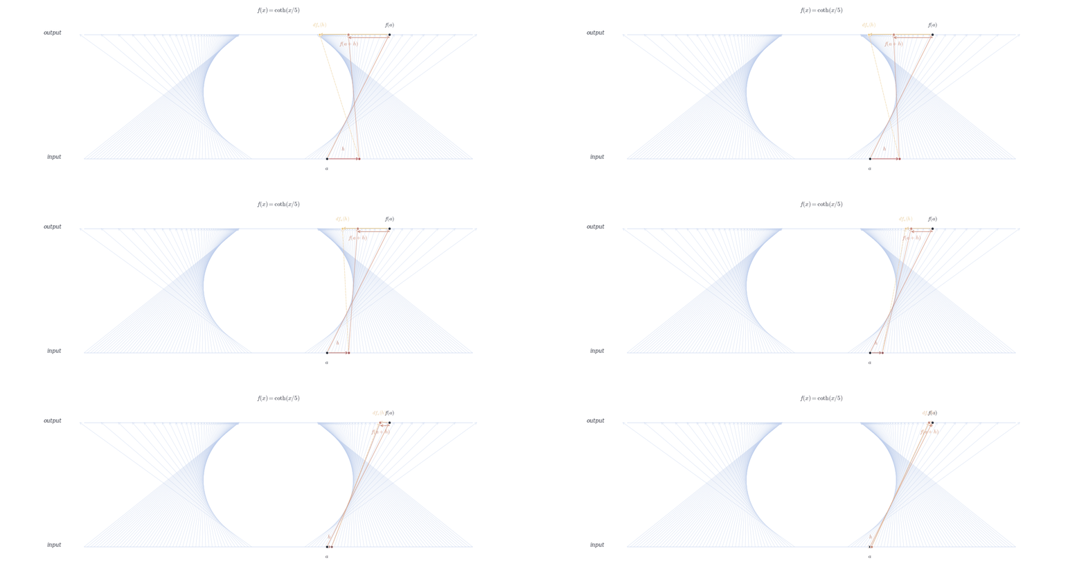
The figure suggests that there exists a point where a differential exactly captures the total change of f over [a,b]. To motivate the construction of an auxiliary function, consider the straight line connecting the endpoints (a,f(a)) and (b,f(b)). Let us define a line L satisfying L(a) = f(a), \qquad L(b) = f(b), so that it passes through the endpoints. By elementary algebra, its slope must be \frac{f(b) - f(a)}{b-a}, and hence L(x) = f(a) + \frac{f(b)-f(a)}{b-a}(x-a).
This line L encodes the “ideal” linear change across the interval. To locate a point where the derivative of f coincides with this ideal slope, it is natural to consider the difference between f and L. This motivates the definition of the auxiliary function \psi(x) = f(x) - L(x), which satisfies \psi(a) = \psi(b) = 0 by construction. The properties of \psi will then guide the identification of a point c \in (a,b) where f'(c) equals the slope of the secant line.
Theorem 9.2 (Mean Value Theorem) Let f : [a,b] \to \mathbb{R} be continuous on [a,b] and differentiable on (a,b). Then there exists c \in (a,b) such that f(b) - f(a) = f'(c)(b - a).
Equivalently, the differential at c captures the total change: f(b) - f(a) = df_c(b - a).
To locate a point where the differential exactly captures the total change, define the auxiliary function as before \psi(x) = f(x) - \Bigl(f(a) + \frac{f(b)-f(a)}{b-a}(x-a)\Bigr) = f(x) - L(x), so that \psi(a) = \psi(b) = 0. This \psi measures the deviation of f from the straight line L connecting the endpoints.
Since \psi is continuous on [a,b] and differentiable on (a,b), Theorem 7.5 guarantees it attains a extremum at some point c \in [a,b]. If the extremum occurs in the interior (which must happen unless \psi:= 0), the differential vanishes d\psi_c(h) = 0 \quad \text{for all } h.
By linearity, d\psi_c(h) = df_c(h) - dL_c(h) = df_c(h) - \frac{f(b)-f(a)}{b-a} h. Choosing h = b-a gives df_c(b-a) = f(b)-f(a), showing that the differential at c exactly reproduces the total change of f over [a,b]. \square
Observe that the following corollary follows immediately from the theorem
Corollary 9.1 (Rolle’s Theorem) Let f : [a,b] \to \mathbb{R} be continuous on [a,b] and differentiable on (a,b). If f(a) = f(b), then there exists c \in (a,b) such that df_c = 0 \quad \text{or equivalently} \quad f'(c) = 0.
Consider the total change f(b)-f(a) = 0. By Theorem 9.2, some differential df_c must exactly capture this change df_c(b-a) = 0. Since b-a \neq 0, it follows that df_c = 0.
9.6 Looking Back: Linear Algebra Revisited
Now that we’ve developed differentiation, let’s revisit the linear algebra concepts from Section 8.3 and see how they manifested
| Linear Algebra Concept | Role in Differentiation |
|---|---|
| Linear map T: \mathbb{R} \to \mathbb{R} | The derivative as an approximation: T(h) = f'(a)h |
| Linear functional \varphi(h) | The differential df_a(h) measures change |
| Norm \|h\| | Measuring displacement to define relative error |
| Composition T \circ S | Chain rule (coming in next chapter) |
| Linear combination | Linearity of differentiation: (af+bg)' = af' + bg' |
Differentiation is a process that extracts a linear map from a nonlinear function. Given f, the derivative operator D produces Df(a) = f'(a), which determines the linear functional df_a(h) = f'(a)h.
Consider the function f(x) = x^3 at the point a = 2.
Use the definition of the derivative (Definition 9.1) to compute f'(2). Specifically, evaluate \lim_{h \to 0} \frac{f(2+h) - f(2)}{h}.
Write the equation of the tangent line to y = x^3 at the point (2, 8).
Use your tangent line from part (b) to estimate f(2.1). Compare this to the actual value and compute the error.
The differential df_2 is a linear functional that approximates the change in f near x=2.
Write df_2(h) = f'(2) \cdot h explicitly using your answer from part (a).
Use df_2(h) to approximate f(2.05) by computing f(2) + df_2(0.05).
Explain why this gives the same result as using the tangent line equation from part (b) with x = 2.05.
Let g(x) = \sqrt{x} for x > 0.
Prove that g'(a) = \frac{1}{2\sqrt{a}} for any a > 0 by computing the limit of the difference quotient. (Hint: Multiply numerator and denominator by the conjugate.)
Show that g is continuous at x = 4 using Theorem 9.1.
Explain geometrically why g'(x) \to \infty as x \to 0^+. What does this say about the tangent line to y = \sqrt{x} near the origin?
In this problem, you will apply the Mean Value Theorem.
Let f(x) = x^2 - 4x + 1 on [1, 4]. Find the point c \in (1, 4) guaranteed by Theorem 9.2 where the tangent line is parallel to the secant line connecting (1, f(1)) and (4, f(4)).
Suppose f is differentiable on [a, b] and f'(x) = 0 for all x \in (a, b). Use Theorem 9.2 to prove that f is constant on [a, b].
Lipschitz continuity. Use Theorem 9.2 to prove that if |f'(x)| \leq M for all x \in [a, b], then |f(b) - f(a)| \leq M|b - a|.
Computing the derivative. We have \frac{f(2+h) - f(2)}{h} = \frac{(2+h)^3 - 8}{h}.
Expanding (2+h)^3 = 8 + 12h + 6h^2 + h^3, we obtain \frac{8 + 12h + 6h^2 + h^3 - 8}{h} = \frac{12h + 6h^2 + h^3}{h} = 12 + 6h + h^2.
Taking the limit as h \to 0, f'(2) = \lim_{h \to 0} (12 + 6h + h^2) = 12.
Tangent line equation. The tangent line at (2, 8) has slope f'(2) = 12 and passes through (2, 8). Using point-slope form: y - 8 = 12(x - 2) y = 12x - 16.
Linear approximation. Using the tangent line to estimate f(2.1): f(2.1) \approx 12(2.1) - 16 = 25.2 - 16 = 9.2.
The actual value is f(2.1) = (2.1)^3 = 9.261.
The error is |9.261 - 9.2| = 0.061.
This demonstrates that the linear approximation f(x) \approx f(a) + f'(a)(x-a) is accurate for small displacements from a, with error proportional to h^2 (the quadratic term we discarded).
The differential as a linear functional.
From part (a), we found f'(2) = 12. The differential df_2 : \mathbb{R} \to \mathbb{R} is the linear functional defined by
df_2(h) = f'(2) \cdot h = 12h.
This is a linear map from displacements h to predicted changes in f. It satisfies the linearity properties: df_2(h_1 + h_2) = df_2(h_1) + df_2(h_2) and df_2(ch) = c \, df_2(h) for all h, h_1, h_2 \in \mathbb{R} and c \in \mathbb{R}.
To approximate f(2.05), we use the displacement h = 0.05 from the base point x = 2. The approximation formula is f(2 + h) \approx f(2) + df_2(h).
Substituting our values: f(2.05) \approx f(2) + df_2(0.05) = 8 + 12(0.05) = 8 + 0.6 = 8.6.
- The tangent line from part (b) is y = 12x - 16. Evaluating at x = 2.05: y = 12(2.05) - 16 = 24.6 - 16 = 8.6. This matches our differential approximation because both represent the same linear approximation. The tangent line equation y - 8 = 12(x - 2) is equivalent to y = f(2) + 12(x-2). Setting h = x - 2 gives y = f(2) + 12h = f(2) + df_2(h). The differential df_2(h) = 12h is simply the coordinate representation of the tangent line’s slope.
Derivative of square root. For a > 0, compute \frac{g(a+h) - g(a)}{h} = \frac{\sqrt{a+h} - \sqrt{a}}{h}.
Multiply numerator and denominator by the conjugate \sqrt{a+h} + \sqrt{a}: \frac{\sqrt{a+h} - \sqrt{a}}{h} \cdot \frac{\sqrt{a+h} + \sqrt{a}}{\sqrt{a+h} + \sqrt{a}} = \frac{(a+h) - a}{h(\sqrt{a+h} + \sqrt{a})} = \frac{1}{\sqrt{a+h} + \sqrt{a}}.
Taking the limit as h \to 0: g'(a) = \lim_{h \to 0} \frac{1}{\sqrt{a+h} + \sqrt{a}} = \frac{1}{2\sqrt{a}}. \quad \square
Continuity via differentiability. Since g is differentiable at x = 4 (we showed g'(4) = \frac{1}{2\sqrt{4}} = \frac{1}{4} exists), by Theorem 9.1, g must be continuous at x = 4.
This is a general principle: differentiability at a point is a stronger condition than continuity at that point.
Behavior near the origin. From part (a), g'(x) = \frac{1}{2\sqrt{x}}. As x \to 0^+, we have g'(x) = \frac{1}{2\sqrt{x}} \to \infty.
Geometrically, this means the tangent line to y = \sqrt{x} becomes increasingly steep as we approach the origin. The graph has a vertical tangent at x = 0—the slope is undefined there because the derivative does not exist (the limit defining g'(0) diverges to infinity).
Finding the MVT point. First compute the endpoints: f(1) = 1 - 4 + 1 = -2, \quad f(4) = 16 - 16 + 1 = 1.
The slope of the secant line is \frac{f(4) - f(1)}{4 - 1} = \frac{1 - (-2)}{3} = 1.
By Theorem 9.2, there exists c \in (1, 4) where f'(c) = 1.
Since f'(x) = 2x - 4, we solve: 2c - 4 = 1 \implies c = \frac{5}{2} = 2.5.
Indeed, c = 2.5 \in (1, 4). At this point, the tangent line is parallel to the secant line.
Constant function theorem. Let x_1, x_2 \in [a, b] with x_1 < x_2. By Theorem 9.2, there exists c \in (x_1, x_2) \subset (a, b) such that f(x_2) - f(x_1) = f'(c)(x_2 - x_1).
Since f'(c) = 0 by hypothesis, we have f(x_2) - f(x_1) = 0 \cdot (x_2 - x_1) = 0.
Therefore f(x_2) = f(x_1) for all x_1, x_2 \in [a, b]. Hence f is constant on [a, b]. \square
Bounded derivative implies Lipschitz condition. Apply Theorem 9.2 to f on [a, b]. There exists c \in (a, b) such that f(b) - f(a) = f'(c)(b - a).
Taking absolute values: |f(b) - f(a)| = |f'(c)||b - a|.
By hypothesis, |f'(x)| \leq M for all x \in [a, b]. In particular, |f'(c)| \leq M. Therefore |f(b) - f(a)| = |f'(c)||b - a| \leq M|b - a|. \quad \square
This result shows that functions with bounded derivatives cannot change too rapidly—the rate of change is controlled by the bound on the derivative.