12 Differentiation Techniques
Let f and g be functions of a real variable for which the derivatives Df and Dg are defined. Up to this point, we have established rules for computing derivatives of explicit functions and their compositions. These rules suffice for many elementary calculations, but in applications one often encounters functions that are defined implicitly, expressions that are products or powers of functions in which logarithmic manipulation is convenient, and situations requiring higher-order derivatives. (You can verify any derivative computation with our derivative calculator.)
In this section, we introduce several techniques that extend the basic theory of differentiation. Each method may be justified rigorously via the principle of linear approximation, as developed in the preceding chapters.
12.1 Implicit Differentiation
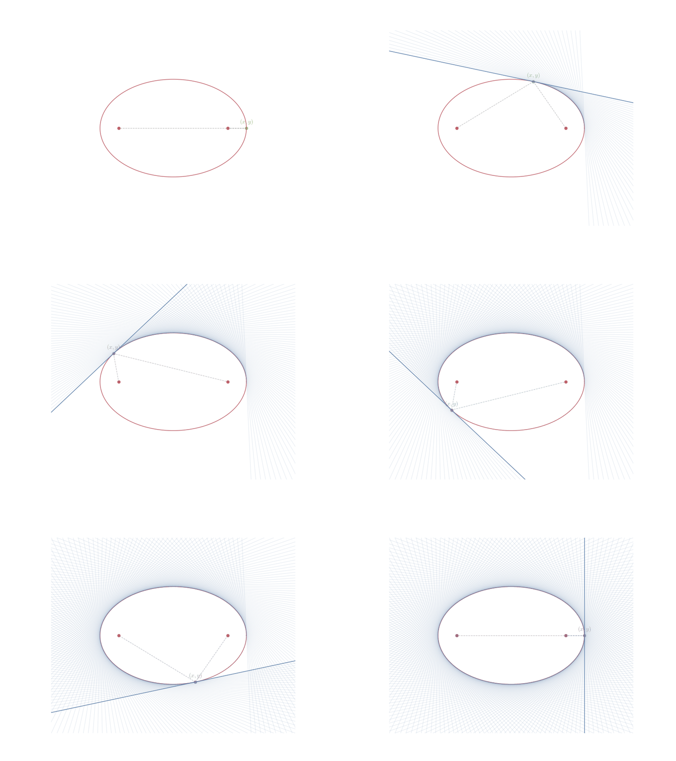
In the early seventeenth century, Kepler studied the motion of planets around the Sun. Observations suggested that planets move along ellipses, with the Sun at one focus. The ellipse with semi-axes a and b is described by the equation
\frac{x^2}{a^2} + \frac{y^2}{b^2} = 1.
Here y is not given as an explicit function of x, yet one often wishes to determine the slope of the tangent line at a point (x,y)—for example, to compute the instantaneous velocity vector of a planet.
Differentiating both sides formally using differentials yields
d\left(\frac{x^2}{a^2} + \frac{y^2}{b^2}\right)(h) = d(1)(h) \implies \frac{2x}{a^2} \, dx(h) + \frac{2y}{b^2} \, dy(h) = 0.
Solving for dy(h) in terms of dx(h), we obtain
dy(h) = -\frac{b^2}{a^2} \cdot \frac{x}{y} \, dx(h).
For a displacement purely along x, we take dx(h) = h, giving the corresponding displacement in y
dy(h) = -\frac{b^2}{a^2}\cdot \frac{x}{y} \, h.
Thus, the linear approximation to y at (x,y) is
y + dy(h) \approx y - \frac{b^2}{a^2} \cdot\frac{x}{y} \, h.
Since the slope of the tangent line is the ratio of the linear changes in y and x, we can write
y' = \frac{dy(h)}{dx(h)} = -\frac{b^2}{a^2} \cdot\frac{x}{y}.

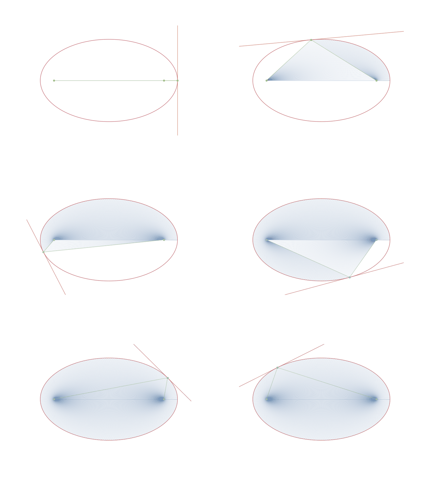
Remark. The ellipse has long attracted mathematical attention. Classically, it is defined as the locus of points whose sum of distances to two fixed points (foci) is constant—a definition already studied by the Greeks. It is likely, however, that such geometric insights were known earlier; the Greeks receive credit (as they do) largely because their work was documented and transmitted. The property that a ray emanating from one focus reflects off the ellipse to pass through the other focus emerges only in later optical and acoustic contexts, when reflective surfaces could be constructed. Subsequently, in applications ranging from mirrors to sound chambers, the geometry of the ellipse was exploited so that waves or rays from one focus converge precisely at the other.

12.1.1 Linear Approximation and Total Differentials
With the geometric motivation above we proceed to the general principle. Let F(x,y) be a differentiable expression in two variables. For a small displacement h in x, one may define the corresponding change in y, denoted dy(h), by requiring that F remains constant to first order:
dF(h) := F(x+h, y+dy(h)) - F(x,y) \approx 0.
Expanding this expression linearly in h gives a relation of the form
\psi(x,y)\, dx(h) + \varphi(x,y)\, dy(h) = 0,
for suitable functions \psi and \varphi determined by F. Note that this is indeed a linear combination of functionals in the sense of Section 8.5: both dx and dy are viewed as maps that take a small displacement h and return a corresponding real number, measuring the first-order change of x and y along that direction. Formally, one may write
L := \psi(x,y)\, dx + \varphi(x,y)\, dy,
as a linear functional on the one-dimensional space of displacements h. In this viewpoint, the expression L no longer depends explicitly on a particular h; it is an abstract linear object. When a specific displacement h is applied, dx and dy act on h to produce the actual infinitesimal changes in x and y, and the relation L(h) = 0 encodes the first-order constraint imposed by the equation F(x,y) = \text{constant}. However, we resume our discussion. Taking dx(h) = h, one may solve for dy(h) dy(h) = -\frac{\psi(x,y)}{\varphi(x,y)}\, dx(h).
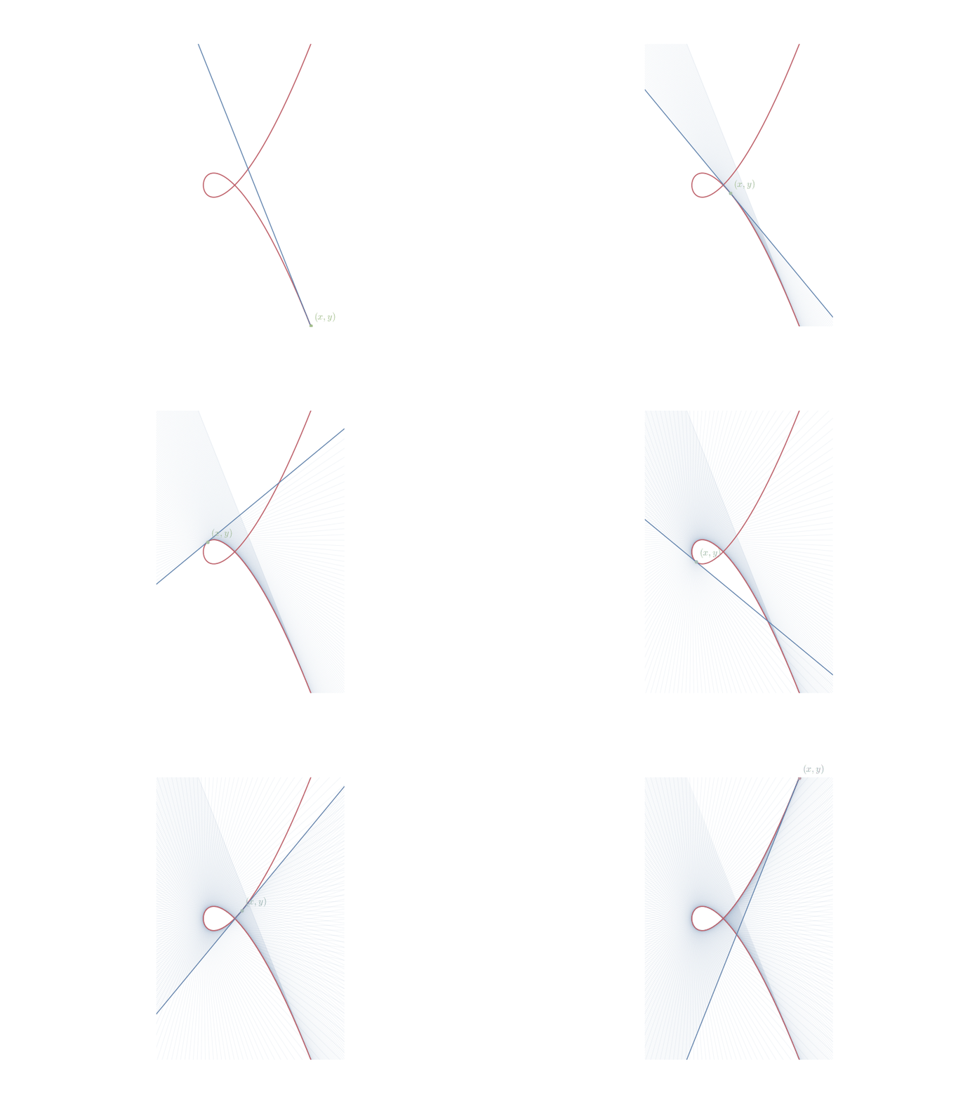
Example 12.1 (The Tschirnhaus’s Cubic) Consider the curve known as the Tschirnhaus’s cubic, defined by the equation y^2 = x^3 + 3x^2.
To determine the slope of the tangent line, we require that the total differential of the function f(x,y) = y^2 - x^3 - 3x^2 remains zero for a small displacement h.
d(y^2)(h) = d(x^3 + 3x^2)(h)
Since y is an implicit function of x, we apply Theorem 10.5 to y^2
d(y^2)(h) = 2y\,dy(h).
We differentiate the polynomial expression in x
d(x^3 + 3x^2)(h) = (3x^2 + 6x)\,dx(h).
Setting the two differential expressions equal, we establish the first-order constraint 2y\,dy(h) = (3x^2 + 6x)\,dx(h).
The derivative y' is the ratio of the change in y to the change in x, which corresponds to the ratio of the linear functionals dy(h) and dx(h). Solving for this ratio gives dy(h)= \frac{3x^2 + 6x}{2y}\,dx(h) Thus, the slope of the tangent line at any point (x,y) on the curve is y' = \frac{3x^2 + 6x}{2y}.

12.2 Logarithmic Differentiation
12.2.1 Motivation: Functions Defined as Products and Powers
Consider a function such as f(x) = x^x.
This is neither a simple power (since the exponent varies) nor an exponential (since the base varies). Direct application of the power rule fails, and the exponential rule does not quite fit. Yet such functions arise naturally in mathematics and statistics—they appear in combinatorics (factorials and their approximations), probability (distributions and likelihood functions), and analysis (growth rates and entropy).
More generally, we often encounter expressions of the form f(x) = [u(x)]^{v(x)}, where both the base u(x) and exponent v(x) depend on x. Computing the derivative directly is cumbersome. However, by taking the natural logarithm, we transform this into an additive structure, revealing a path forward through Theorem 10.5.
The method of logarithmic differentiation is particularly useful when:
A function is written as a product or quotient of several factors
A function involves a variable base and exponent
Algebraic simplification via logarithms reduces complexity
12.2.2 The Method
Suppose f(x) > 0 on some interval. The key insight is to differentiate \ln f(x) rather than f(x) directly. By Theorem 10.5,
\frac{d}{dx} \ln f(x) = \frac{f'(x)}{f(x)}.
Rearranging, we obtain the logarithmic derivative: f'(x) = f(x) \cdot \frac{d}{dx} \ln f(x).
This expresses the derivative of f in terms of the derivative of its logarithm, multiplied by f itself. The derivative of the logarithm often simplifies through properties of logarithms.
12.2.2.1 Example
Compute the derivative of f(x) = x^x for x > 0.
Solution. Taking the natural logarithm, \ln f(x) = \ln(x^x) = x \ln x.
Differentiate both sides with respect to x. On the left, \frac{d}{dx} \ln f(x) = \frac{f'(x)}{f(x)}.
On the right, using the product rule, \frac{d}{dx}(x \ln x) = 1 \cdot \ln x + x \cdot \frac{1}{x} = \ln x + 1.
Equating the two expressions, \frac{f'(x)}{f(x)} = \ln x + 1.
Solve for f'(x): f'(x) = f(x)(\ln x + 1) = x^x(\ln x + 1).
Verification. At x = 1, we have f(1) = 1^1 = 1 and f'(1) = 1 \cdot (\ln 1 + 1) = 1 \cdot 1 = 1. Geometrically, the curve y = x^x has slope 1 at the point (1, 1), consistent with our result.
12.2.2.2 Example
Compute the derivative of f(x) = \frac{(x+1)^3 (x-2)^2}{(x^2+1)^4}.
Solution. Taking logarithms, \ln f(x) = 3 \ln(x+1) + 2 \ln(x-2) - 4 \ln(x^2+1).
Differentiate term-by-term: \frac{f'(x)}{f(x)} = \frac{3}{x+1} + \frac{2}{x-2} - \frac{4 \cdot 2x}{x^2+1} = \frac{3}{x+1} + \frac{2}{x-2} - \frac{8x}{x^2+1}.
Thus, f'(x) = \frac{(x+1)^3 (x-2)^2}{(x^2+1)^4} \left( \frac{3}{x+1} + \frac{2}{x-2} - \frac{8x}{x^2+1} \right).
Remark. Logarithmic differentiation transforms a product into a sum, and a quotient into a difference—operations that are far simpler to differentiate. This is the power of the logarithm: it linearizes multiplication, making complicated expressions tractable.
12.3 Higher-Order Derivatives
12.3.1 Definition and Notation
If f is differentiable at each point of an interval, its derivative Df is itself a function. If Df is also differentiable, we may differentiate it again, obtaining the second differential and the second derivative D^2f. Proceeding inductively, we obtain higher-order differentials and derivatives.
Definition 12.1 (Higher-Order Differentials and Derivatives) Let f be a function differentiable on an interval I. If Df exists and is itself differentiable at a point a, we define the second differential at a by d^2 f_a(h) := D(Df)_a(h).
More generally, the n-th differential is defined recursively: d^n f_a(h) := D(d^{n-1}f)_a(h), \quad n \geq 2.
The n-th derivative at a is the scalar coefficient D^n f(a) satisfying d^n f_a(h) = D^n f(a) \cdot h, in the sense of a linear map. When evaluating the n-th order Taylor approximation, the relevant quantity is D^n f(a) \cdot h^n / n!, but the differential itself is linear in h. The notation \frac{d^n f}{dx^n}\bigg|_{x=a} is also used.
12.3.1.1 Example
For f(x) = x^4 - 3x^2 + 5, \begin{align*} Df(x) &= 4x^3 - 6x, \\ D^2 f(x) &= 12x^2 - 6, \\ D^3 f(x) &= 24x, \\ D^4 f(x) &= 24, \\ D^5 f(x) &= 0. \end{align*}
Beyond the fifth derivative, all higher derivatives vanish. This is typical for polynomials: a polynomial of degree n has D^n f as a nonzero constant, but D^{n+1} f = 0.
12.3.2 Smoothness Classes
The existence of higher derivatives imposes increasingly restrictive conditions on functions. A function may be differentiable once but fail to have a second derivative. Or it may be twice differentiable but not three times. This motivates a classification by degree of smoothness.
Definition 12.2 (C^k Spaces) Let I be an interval. A function f : I \to \mathbb{R} is said to be of class C^k on I if f is k-times continuously differentiable on I. That is:
- f, Df, D^2 f, \ldots, D^{k} f all exist and are continuous on I
We write f \in C^k(I) to indicate that f is of class C^k on I.
Special cases: - C^0(I): continuous functions on I - C^1(I): continuously differentiable functions (differential exists and is continuous) - C^2(I): twice continuously differentiable (second differential exists and is continuous) - C^\infty(I): infinitely differentiable or smooth functions (all derivatives exist)
Hierarchy. We have inclusions C^\infty(I) \subset \cdots \subset C^2(I) \subset C^1(I) \subset C^0(I). Every smooth function is continuously differentiable, but not every continuously differentiable function is twice differentiable. For instance, f(x) = x^{3/2} is C^1 on [0,\infty) but not C^2 at x = 0, since D^2 f(x) = \frac{3}{4\sqrt{x}} is unbounded near 0.
Examples: - Polynomials are C^\infty(\mathbb{R}) - e^x, \sin x, \cos x are C^\infty(\mathbb{R}) - |x| is C^0(\mathbb{R}) but not C^1(\mathbb{R}) (not differentiable at 0) - f(x) = \begin{cases} x^2 \sin(1/x) & x \neq 0 \\ 0 & x = 0 \end{cases} is C^1(\mathbb{R}) but not C^2(\mathbb{R}) (derivative exists but is discontinuous at 0)
Remark. The requirement that derivatives be continuous is essential. A function can have derivatives that exist everywhere but are discontinuous. Such pathological examples motivate the distinction between “differentiable” and “C^1.”
In what follows, when we say a function is smooth, we mean f \in C^\infty—infinitely differentiable with all derivatives continuous. This is the natural class of functions for Taylor series and asymptotic analysis.
12.3.3 Linearity of Higher-Order Differentiation
Just as the first differential is linear, higher-order differentials inherit linearity from the definition.
Theorem 12.1 (Higher-Order Derivatives Respect Linearity) Let f and g be n-times differentiable at a, and let c \in \mathbb{R}. Then:
- D^n(f + g)(a) = D^n f(a) + D^n g(a)
- D^n(cf)(a) = c \cdot D^n f(a)
We proceed by induction. The base case n = 1 follows from the linearity of the first differential (see Theorem 10.1 and Theorem 10.2).
Assume the result holds for n - 1. Then D^n(f+g)(a) = D(D^{n-1}(f+g))(a) = D(D^{n-1}f + D^{n-1}g)(a).
By the inductive hypothesis, D^{n-1}(f+g) = D^{n-1}f + D^{n-1}g. Now apply the base case to obtain D(D^{n-1}f + D^{n-1}g)(a) = D(D^{n-1}f)(a) + D(D^{n-1}g)(a) = D^n f(a) + D^n g(a).
The scalar multiplication case is analogous. \square
12.3.4 The Second Differential and Concavity
The second differential provides geometric information about the curvature of a function. Recall that at a point a, the first differential df_a(h) = Df(a) \cdot h encodes how f changes linearly under small displacements h. The second differential measures how this linear approximation itself changes.
More precisely, the difference between the actual function and its linear approximation is E_1(h) = f(a+h) - f(a) - df_a(h) = o(h).
For small h, this error is small—but what drives its shape? The second differential provides this answer. We have f(a+h) = f(a) + df_a(h) + \frac{1}{2} d^2 f_a(h) + o(h^2), where the quadratic term \frac{1}{2} d^2 f_a(h) = \frac{1}{2} D^2 f(a) h^2 dominates the next-order behavior.
Definition 12.3 (Concavity) A function f is concave up at a point a if D^2 f(a) > 0. It is concave down at a if D^2 f(a) < 0. A point a where D^2 f(a) = 0 and D^2 f changes sign nearby is called an inflection point.
Interpretation. If D^2 f(a) > 0, the second differential d^2 f_a(h) = D^2 f(a) h^2 is positive for all h \neq 0. This means the function curves upward: the graph lies above its tangent line near a. Conversely, if D^2 f(a) < 0, the function curves downward.
Physical Interpretation. If s(t) represents position at time t, then v(t) = Ds(t) is velocity, and a(t) = D^2s(t) is acceleration. A positive acceleration means the velocity is increasing; a negative acceleration means it is decreasing.
12.3.5 Curvature and the Ellipse Revisited
Having seen how the second differential d^2f measures concavity, we now develop the tools to compute curvature—the intrinsic bending of a curve, independent of parameterization. This requires first deriving the arc length element. We return to Kepler’s ellipse to see how second derivatives encode both geometric and dynamical information.
Consider a small displacement h along the x-axis. This induces a displacement vector in the plane: \mathbf{v}(h) = \begin{pmatrix} dx(h) \\ dy(h) \end{pmatrix} = \begin{pmatrix} h \\ Df(x) \cdot h \end{pmatrix}, where dx(h) = h is the horizontal displacement and dy(h) = df(h) = Df(x) \cdot h is the corresponding vertical displacement along the curve y = f(x).
The magnitude (or length) of this displacement vector is the arc length element. Using the Euclidean norm from the vector space structure on \mathbb{R}^2, we have \|\mathbf{v}(h)\| = \sqrt{(dx(h))^2 + (dy(h))^2} = \sqrt{h^2 + (Df(x) \cdot h)^2} = |h| \sqrt{1 + (Df(x))^2}.
For an infinitesimal displacement h = dx, the infinitesimal arc length is ds = \sqrt{(dx)^2 + (df)^2} = \sqrt{1 + (Df(x))^2} \, dx.
The arc length ds = \sqrt{(dx)^2 + (dy)^2} combines horizontal and vertical displacements into a single geometric quantity: the actual distance traversed. This is the magnitude of the displacement vector \mathbf{v} = (dx, dy) in the tangent space.
The curvature \kappa is the rate at which the tangent angle changes per unit arc length. For a curve y = f(x), the tangent angle \theta satisfies \tan \theta = Df(x), so \frac{d\theta}{dx} = \frac{D^2 f(x)}{1 + (Df(x))^2}.
To get the change per unit arc length, divide by ds/dx = \sqrt{1 + (Df(x))^2}:
Definition 12.4 (Curvature) The curvature of a curve y = f(x) is \kappa = \frac{|D^2 f(x)|}{(1 + (Df(x))^2)^{3/2}}.
The absolute value ensures curvature is always non-negative. The denominator accounts for the curve’s steepness: a nearly vertical curve (large |Df|) traverses a long arc length for small dx, so the curvature is diminished relative to the second derivative.
At points where the curve is horizontal (Df(x) = 0), the curvature simplifies to \kappa = |D^2 f(x)|. Here the second derivative directly measures the bending.
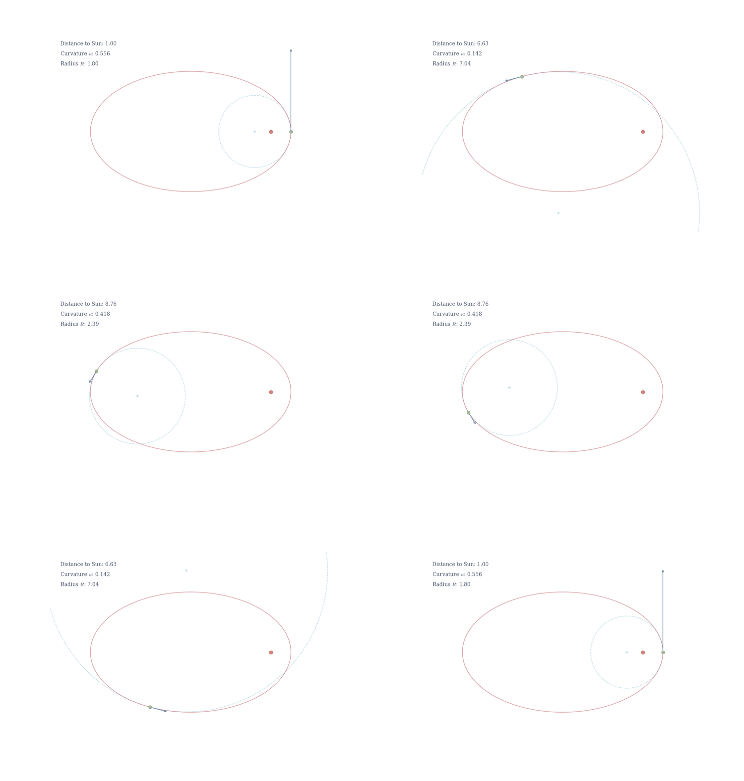
The reciprocal R = 1/\kappa is the radius of curvature—the radius of the circle that best approximates the curve at that point. A small radius means tight bending (high curvature); a large radius means gentle bending (low curvature).
Example 12.2 (Curvature of Kepler’s Ellipse) We apply these formulas to the ellipse from our earlier discussion. Consider the ellipse given by \frac{x^2}{a^2} + \frac{y^2}{b^2} = 1, where a > b > 0. We solve for y in the upper half: y = b\sqrt{1 - \frac{x^2}{a^2}}.
The first derivative, via the chain rule: \frac{dy}{dx} = b \cdot \frac{1}{2\sqrt{1 - x^2/a^2}} \cdot \left(-\frac{2x}{a^2}\right) = -\frac{bx}{a^2\sqrt{1 - x^2/a^2}}.
The second derivative (using the quotient rule and chain rule): \frac{d^2y}{dx^2} = -\frac{b}{a^2} \cdot \frac{d}{dx}\left[\frac{x}{\sqrt{1 - x^2/a^2}}\right].
After differentiation: \frac{d^2y}{dx^2} = -\frac{b}{a^2} \cdot \frac{\sqrt{1 - x^2/a^2} - x \cdot \frac{-x/a^2}{\sqrt{1 - x^2/a^2}}}{1 - x^2/a^2} = -\frac{b}{a^2(1 - x^2/a^2)^{3/2}}.
At the top of the ellipse (x = 0, y = b), this simplifies to \frac{d^2y}{dx^2}\bigg|_{x=0} = -\frac{b}{a^2}.
The negative sign confirms the ellipse is concave down at its peak. At this point, the tangent is horizontal (dy/dx = 0), so the curvature formula reduces to \kappa = \left|\frac{d^2y}{dx^2}\right| = \frac{b}{a^2}.
At the side of the ellipse (a, 0), by symmetry, the curvature is \kappa = a/b^2.
Kepler’s first law states that planets orbit in ellipses with the Sun at one focus. A planet moves fastest approaching the Sun and slowest at farthest point. This follows from conservation of angular momentum: r^2 \frac{d\theta}{dt} = \text{constant}, where r is the distance from the Sun and \theta is the angular position.

Geometrically, this is related to curvature. Near the narrow end of the ellipse (the focus), the orbit curves sharply—high curvature corresponds to tight bending and rapid angular motion. At the wide end, the curvature is gentler, and the planet moves more slowly. In general relativity, gravity itself is the curvature of spacetime. Planets follow geodesics—the shortest possible paths—in curved space. What physicists call “gravitational acceleration” is simply the manifestation of moving along a curved trajectory in curved space.
12.4 The Inverse Function Theorem
12.4.1 Motivation: Reversing Differentiation
Suppose a function f is invertible on an interval I, meaning there exists a function f^{-1} such that f(f^{-1}(x)) = x for all x in the range of f. If f is differentiable and f'(a) \neq 0 at a point a, what can we say about the derivative of f^{-1}?
The answer is intuitive: if f is “stretching” space by a factor of f'(a) near a, then f^{-1} must be “compressing” by the reciprocal factor. More precisely,
\left(f^{-1}\right)'(b) = \frac{1}{f'(a)},
where b = f(a).
This relationship is the inverse function theorem in one dimension.
12.4.2 Statement and Proof
Theorem 12.2 (Inverse Function Theorem (One Dimension).) Let f be differentiable on an interval I, and suppose Df(a) \neq 0 at some point a \in I. Then f is locally invertible near a, and the inverse function f^{-1} is differentiable at b = f(a). Its differential is d(f^{-1})_b(k) = \frac{k}{Df(a)}, so that D(f^{-1})(b) = \frac{1}{Df(a)}.
By definition of inverse, f^{-1}(f(x)) = x for all x in a neighborhood of a. The identity function has differential d(x)_x(h) = h.
Applying Theorem 10.5 to f^{-1}(f(x)) = x, we have at a point x near a, d(f^{-1})_{f(x)}(df_x(h)) = h.
Setting h' = df_x(h) = Df(x) \cdot h, we obtain d(f^{-1})_{f(x)}(h') = \frac{h'}{Df(x)}.
At the point x = a, let b = f(a) and k = h'. Then d(f^{-1})_b(k) = \frac{k}{Df(a)}.
Thus D(f^{-1})(b) = \frac{1}{Df(a)}. \square
12.4.3 Applications: Derivatives of Inverse Trigonometric Functions
The inverse function theorem immediately gives us derivatives of inverse trigonometric functions via the differential framework.
12.4.3.1 Arcsine
Consider f(x) = \sin x on \left[-\frac{\pi}{2}, \frac{\pi}{2}\right], where it is one-to-one with inverse f^{-1}(y) = \arcsin(y) for y \in [-1,1].
We have Df(x) = \cos x. On the open interval \left(-\frac{\pi}{2}, \frac{\pi}{2}\right), \cos x > 0. By the inverse function theorem, for b = \sin x with x \in \left(-\frac{\pi}{2}, \frac{\pi}{2}\right), D(\arcsin)(b) = \frac{1}{\cos x}.
To express this in terms of b, use \sin^2 x + \cos^2 x = 1: \cos x = \sqrt{1 - \sin^2 x} = \sqrt{1 - b^2}.
Therefore, for y \in (-1, 1), \boxed{D(\arcsin)(y) = \frac{1}{\sqrt{1-y^2}}.}
Or in standard notation, \frac{d}{dx}\arcsin x = \frac{1}{\sqrt{1-x^2}}.
12.4.3.2 Arctangent
Consider f(x) = \tan x on \left(-\frac{\pi}{2}, \frac{\pi}{2}\right). Its inverse is f^{-1}(y) = \arctan(y) for all y \in \mathbb{R}.
We have Df(x) = \sec^2 x = 1 + \tan^2 x. At a point where y = \tan x, D(\arctan)(y) = \frac{1}{1 + \tan^2 x} = \frac{1}{1 + y^2}.
Thus, \boxed{\frac{d}{dx}\arctan x = \frac{1}{1+x^2}.}
12.4.3.3 Arccosine and Inverse Hyperbolic Functions
By similar reasoning on [0, \pi] where cosine is decreasing, \frac{d}{dx}\arccos x = -\frac{1}{\sqrt{1-x^2}}.
The negative sign arises because D(\cos x) = -\sin x < 0 on (0, \pi).
For inverse hyperbolic functions, the same method applies. For instance, \frac{d}{dx}\operatorname{arsinh} x = \frac{1}{\sqrt{1+x^2}}.
Consider the curve defined implicitly by x^3 + y^3 = 6xy.
Use implicit differentiation to compute dy/dx in terms of x and y.
Find the points on the curve where the tangent line is horizontal.
Let f(x) = (\sin x)^x for x \in (0, \pi).
Use logarithmic differentiation to compute Df(x).
Determine the critical points of f in (0, \pi).
Let g(x) = e^{-1/x^2} for x \neq 0 and g(0) = 0.
Show that Dg(0) = 0.
Prove that D^n g(0) = 0 for all n \in \mathbb{N}.
Let f : (0, \infty) \to (0, \infty) be differentiable and invertible with f(2) = 3 and Df(2) = 5.
Compute D(f^{-1})(3).
If additionally D^2f(2) = 7, find D^2(f^{-1})(3) by differentiating the identity f^{-1}(f(x)) = x.
Differentiate both sides with respect to x: d(x^3 + y^3) = d(6xy) \implies 3x^2 dx + 3y^2 dy = 6y \, dx + 6x \, dy. Collecting terms with dy: (3y^2 - 6x) dy = (6y - 3x^2) dx. Thus \frac{dy}{dx} = \frac{6y - 3x^2}{3y^2 - 6x} = \frac{2y - x^2}{y^2 - 2x}.
The tangent line is horizontal when dy/dx = 0, requiring 2y - x^2 = 0 with y^2 - 2x \neq 0. Substituting y = x^2/2 into the original equation: x^3 + \frac{x^6}{8} = 6x \cdot \frac{x^2}{2} = 3x^3. Simplifying: x^6 = 16x^3, so x^3(x^3 - 16) = 0. Since we need x > 0 (to avoid y^2 - 2x = 0), we have x = 2\sqrt[3]{2} and y = 4\sqrt[3]{4}.
Taking logarithms: \ln f(x) = x \ln(\sin x). Differentiate: \frac{Df(x)}{f(x)} = \ln(\sin x) + x \cdot \frac{\cos x}{\sin x} = \ln(\sin x) + x \cot x. Thus Df(x) = (\sin x)^x [\ln(\sin x) + x \cot x].
Critical points occur when Df(x) = 0. Since (\sin x)^x > 0, we require \ln(\sin x) + x \cot x = 0. This is a transcendental equation with no closed-form solution. Numerical methods show a critical point near x \approx 2.33.
By definition, Dg(0) = \lim_{h \to 0} \frac{g(h) - g(0)}{h} = \lim_{h \to 0} \frac{e^{-1/h^2}}{h}. Substituting u = 1/h^2, as h \to 0, we have u \to \infty, and \frac{e^{-1/h^2}}{h} = \frac{1}{h e^{1/h^2}} = \frac{u^{1/2}}{e^u} \to 0 since exponentials dominate power functions. Thus Dg(0) = 0.
We proceed by induction. The base case n = 1 was shown in part (a).
For x \neq 0, compute Dg(x) using the chain rule: Dg(x) = e^{-1/x^2} \cdot \frac{2}{x^3} = \frac{2}{x^3} e^{-1/x^2}.
Inductive step. Assume D^k g(x) = P_k(1/x) e^{-1/x^2} for some polynomial P_k when x \neq 0. Differentiating using the product and chain rules: D^{k+1} g(x) = \left[P_k'(1/x) \cdot \left(-\frac{1}{x^2}\right) + P_k(1/x) \cdot \frac{2}{x^3}\right] e^{-1/x^2}.
Both terms are of the form Q(1/x) e^{-1/x^2} for some polynomial Q, establishing the form for D^{k+1} g.
Now we show D^n g(0) = 0 for all n. Given that D^{n-1} g(x) = P_{n-1}(1/x) e^{-1/x^2} and D^{n-1} g(0) = 0 (inductive hypothesis), we have D^n g(0) = \lim_{h \to 0} \frac{P_{n-1}(1/h) e^{-1/h^2}}{h}.
Since P_{n-1}(1/h) is a polynomial in 1/h, say of degree m, this is \lim_{h \to 0} \frac{c_m h^{-m} + \cdots + c_0}{h \cdot e^{1/h^2}} = \lim_{u \to \infty} \frac{c_m u^{m/2} + \cdots}{e^u} = 0, where u = 1/h^2. The exponential dominates any polynomial, so D^n g(0) = 0. \square
By Theorem 12.2, D(f^{-1})(3) = \frac{1}{Df(2)} = \frac{1}{5}.
Differentiate f^{-1}(f(x)) = x using Theorem 10.5: D(f^{-1})(f(x)) \cdot Df(x) = 1. Differentiate again using Theorem 10.4: D^2(f^{-1})(f(x)) \cdot [Df(x)]^2 + D(f^{-1})(f(x)) \cdot D^2f(x) = 0. At x = 2: D^2(f^{-1})(3) \cdot 25 + \frac{1}{5} \cdot 7 = 0. Thus D^2(f^{-1})(3) = -\frac{7}{125}.