6 Asymptotic Behavior and Limits at Infinity

6.1 Motivation

The \varepsilon-\delta formalism treats limits as x approaches a finite point a. Many applications, however, require understanding the behavior of functions as the argument grows without bound.

Consider gravitational force. Newton’s law of universal gravitation states that the force between two masses m_1 and m_2 separated by distance r is

F(r) = \frac{Gm_1m_2}{r^2},

where G is the gravitational constant. As the distance r \to \infty, the force decays to zero—objects infinitely far apart exert no gravitational influence on each other. Similarly, other inverse square laws in physics—electrostatic and radiative intensity—exhibit the same limiting behavior. These observations demand a rigorous notion of limits at infinity.

Beyond computing such limits, we establish a growth hierarchy. Logarithmic functions grow slower than polynomial functions, which grow slower than exponential functions. This hierarchy is fundamental to algorithm analysis, asymptotic expansions, and the study of differential equations.

Finally, we introduce little-o notation, which provides concise language for comparing rates of growth. This formalism appears throughout analysis, probability, and numerical methods.

6.2 Limits at Infinity

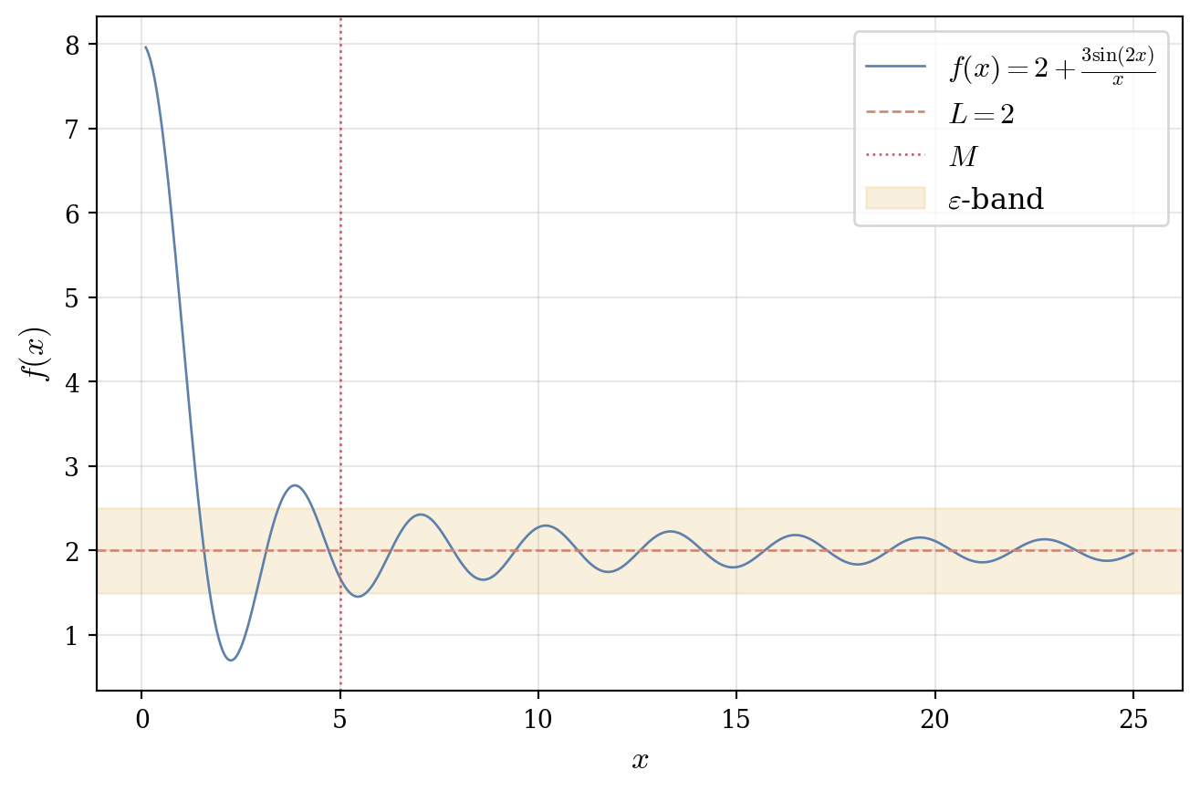
Definition 6.1 (Limit at Infinity) We write \lim_{x \to \infty} f(x) = L if for every \varepsilon > 0, there exists M > 0 such that

x > M \implies |f(x) - L| < \varepsilon.

The definition replaces “|x - a| < \delta” with “x > M”, adapting the \varepsilon-\delta framework to infinite limits. Eventually, f(x) lies within \varepsilon of L.

6.2.0.1 Example

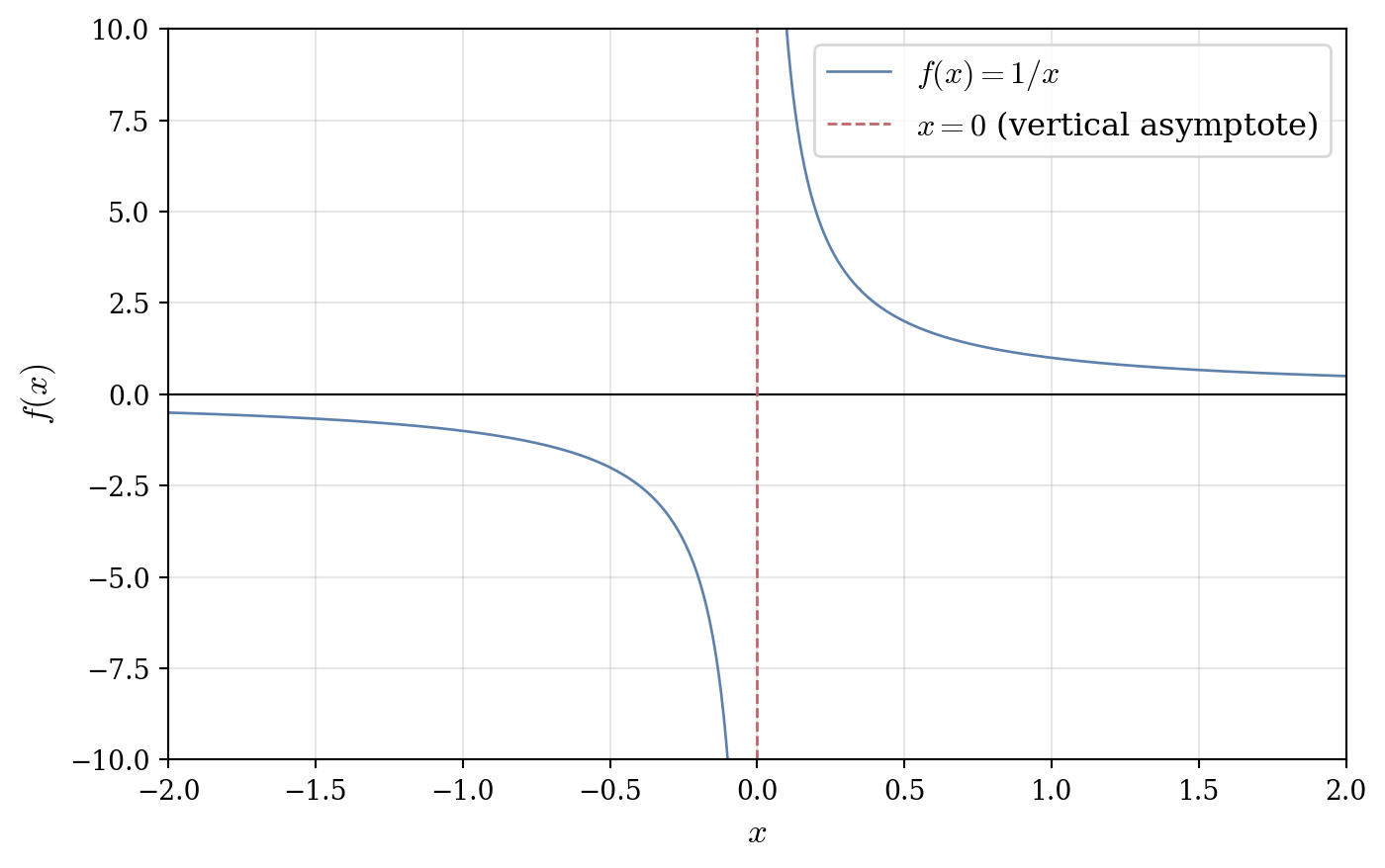
For f(x) = \frac{1}{x}, given \varepsilon > 0, choose M = \frac{1}{\varepsilon}. Then x > M implies

\left|\frac{1}{x}\right| < \frac{1}{M} = \varepsilon.

Hence \lim_{x \to \infty} \frac{1}{x} = 0.

Definition 6.2 (Limit at Negative Infinity) We write \lim_{x \to -\infty} f(x) = L if for every \varepsilon > 0, there exists M < 0 such that

x < M \implies |f(x) - L| < \varepsilon.

Remark. Limits as x \to \infty and x \to -\infty are independent; a function may possess one but not the other.

6.3 Infinite Limits

We formalize unbounded growth.

Definition 6.3 (Infinite Limit) We write \lim_{x \to a} f(x) = \infty if for every N > 0, there exists \delta > 0 such that

0 < |x - a| < \delta \implies f(x) > N.

Similarly, \lim_{x \to a} f(x) = -\infty if for every N < 0, there exists \delta > 0 such that

0 < |x - a| < \delta \implies f(x) < N.

6.3.0.1 Example

For f(x) = \frac{1}{(x-2)^2} and any N > 0, choose \delta = \frac{1}{\sqrt{N}}. Then 0 < |x - 2| < \delta implies

f(x) = \frac{1}{(x-2)^2} > \frac{1}{\delta^2} = N.

Hence \lim_{x \to 2} f(x) = \infty. We say x = 2 is a vertical asymptote. If \lim_{x \to \infty} f(x) = L, then y = L is a horizontal asymptote.

6.4 Asymptotic Behavior of Rational Functions

Limits of rational functions at infinity are determined by the degrees of numerator and denominator.

Theorem 6.1 (Rational Functions at Infinity) Let p(x) = a_n x^n + \cdots + a_0 and q(x) = b_m x^m + \cdots + b_0 with a_n, b_m \neq 0. Then

If n < m: \displaystyle \lim_{x \to \infty} \frac{p(x)}{q(x)} = 0.
If n = m: \displaystyle \lim_{x \to \infty} \frac{p(x)}{q(x)} = \frac{a_n}{b_m}.
If n > m: \displaystyle \lim_{x \to \infty} \frac{p(x)}{q(x)} = \pm \infty (sign determined by a_n, b_m).

Proof

Factor out the highest powers:

\frac{p(x)}{q(x)} = x^{n-m} \frac{a_n + a_{n-1}/x + \cdots + a_0/x^n}{b_m + b_{m-1}/x + \cdots + b_0/x^m}.

As x \to \infty, all terms with 1/x^k vanish. The numerator approaches a_n, the denominator approaches b_m.

If n < m, then x^{n-m} \to 0, yielding limit 0.

If n = m, then x^{n-m} = 1, yielding limit a_n/b_m.

If n > m, then x^{n-m} \to \infty, yielding \pm\infty according to the signs of a_n and b_m. \square

Example 6.1 (Limit of a Rational Function) Evaluate \displaystyle \lim_{x \to \infty} \frac{3x^2 + 5x - 1}{2x^2 + 7}.

Solution

The degrees are equal (n = m = 2), so by Theorem 6.1,

\lim_{x \to \infty} \frac{3x^2 + 5x - 1}{2x^2 + 7} = \frac{3}{2}.

Alternatively, divide numerator and denominator by x^2

\frac{3x^2 + 5x - 1}{2x^2 + 7} = \frac{3 + \frac{5}{x} - \frac{1}{x^2}}{2 + \frac{7}{x^2}}.

As x \to \infty, the fractions vanish

\lim_{x \to \infty} \frac{3 + \frac{5}{x} - \frac{1}{x^2}}{2 + \frac{7}{x^2}} = \frac{3 + 0 - 0}{2 + 0} = \frac{3}{2}. \quad \square

6.5 Growth Hierarchies

Functions exhibit different rates of growth as x \to \infty. We formalize this via dominance.

Definition 6.4 (Dominance) We say f dominates g as x \to \infty, written f \gg g, if

\lim_{x \to \infty} \frac{g(x)}{f(x)} = 0.

Theorem 6.2 (Standard Growth Rates) As x \to \infty:

For a > b > 0: x^a \gg x^b.
For any n \in \mathbb{N}: e^x \gg x^n.
For any a > 0: x^a \gg \ln x.

More explicitly,

\lim_{x \to \infty} \frac{\ln x}{x^a} = 0, \quad \lim_{x \to \infty} \frac{x^n}{e^x} = 0

Remark. These results are proved via L’Hôpital’s Rule in Section 14.6. The complete hierarchy is

\log(\log x) \ll \log x \ll x^{1/n} \ll x \ll x \log x \ll x^2 \ll x^n \ll e^x \ll e^{x^2} \ll e^{e^x}.

6.6 Indeterminate Forms at Infinity

Just as \frac{0}{0} is indeterminate at finite points, forms like \frac{\infty}{\infty}, 0 \cdot \infty, and \infty - \infty are indeterminate at infinity.

6.6.1 Type \frac{\infty}{\infty}

Example 6.2 (Type \frac{\infty}{\infty}) Evaluate \displaystyle \lim_{x \to \infty} \frac{5x^3 - x}{2x^3 + 7}.

Solution

Divide by x^3:

\frac{5x^3 - x}{2x^3 + 7} = \frac{5 - \frac{1}{x^2}}{2 + \frac{7}{x^3}} \to \frac{5}{2}. \quad \square

6.6.2 Type 0 \cdot \infty

Example 6.3 (Type 0 \cdot \infty) Evaluate \displaystyle \lim_{x \to 0^+} x \ln x.

Solution

Rewrite as x \ln x = \frac{\ln x}{1/x}, producing \frac{-\infty}{\infty}. L’Hôpital’s Rule (see ?sec-lhopital) yields 0. \square

6.6.3 Type \infty - \infty

When two terms both approach infinity but with opposite signs, the limit is indeterminate. Techniques include finding a common denominator or using conjugate multiplication.

Example 6.4 (Indeterminate Form \infty - \infty) Evaluate \displaystyle \lim_{x \to \infty} \left(\sqrt{x^2 + x} - x\right).

Solution

As x \to \infty, both terms approach \infty, giving \infty - \infty. Multiply by the conjugate

\begin{align*} \sqrt{x^2 + x} - x &= \left(\sqrt{x^2 + x} - x\right) \cdot \frac{\sqrt{x^2 + x} + x}{\sqrt{x^2 + x} + x} \\ &= \frac{(x^2 + x) - x^2}{\sqrt{x^2 + x} + x} \\ &= \frac{x}{\sqrt{x^2 + x} + x}. \end{align*}

Divide numerator and denominator by x (assuming x > 0)

\frac{x}{\sqrt{x^2 + x} + x} = \frac{1}{\sqrt{1 + \frac{1}{x}} + 1}.

As x \to \infty, \frac{1}{x} \to 0, so

\lim_{x \to \infty} \left(\sqrt{x^2 + x} - x\right) = \frac{1}{\sqrt{1 + 0} + 1} = \frac{1}{2}. \quad \square

6.7 Little-o Notation

Landau’s asymptotic notation provides concise language for relative growth rates.

Definition 6.5 (Little-o) Let f, g be functions and a \in \mathbb{R} \cup \{\pm\infty\}. We write

f(x) = o(g(x)) \quad \text{as } x \to a

\lim_{x \to a} \frac{f(x)}{g(x)} = 0.

6.7.0.1 Examples:

x^2 = o(x) as x \to 0. By definition, we must show \lim_{x \to 0} \frac{x^2}{x} = 0. Simplifying: \lim_{x \to 0} \frac{x^2}{x} = \lim_{x \to 0} x = 0.
\ln x = o(x) as x \to \infty. We must show \lim_{x \to \infty} \frac{\ln x}{x} = 0. This follows from the growth hierarchy (Theorem 14.3): logarithmic functions grow slower than any positive power of x.
e^{-x} = o(x^{-n}) as x \to \infty for any n. We must show \lim_{x \to \infty} \frac{e^{-x}}{x^{-n}} = 0. Rewrite: \frac{e^{-x}}{x^{-n}} = \frac{x^n}{e^x}. By the growth hierarchy, exponential functions dominate all polynomials, so \lim_{x \to \infty} \frac{x^n}{e^x} = 0.

Example 6.5 (Little-o and Thermal Equilibrium) Newton’s law of cooling states that the temperature difference T(t) - T_{\text{env}} between an object and its environment decays exponentially. For small time intervals near t = 0, we can approximate the exponential decay. Specifically, if an object starts at temperature T_0 in an environment at temperature T_{\text{env}}, the temperature difference satisfies

T(t) - T_{\text{env}} = (T_0 - T_{\text{env}})e^{-kt}

for some cooling constant k > 0. For small t, the exponential can be approximated: e^{-kt} \sim 1 - kt. The error in this approximation is o(t). Verify this.

Solution

We must show that e^{-kt} - (1 - kt) = o(t) as t \to 0. By definition of little-o, this requires

\lim_{t \to 0} \frac{e^{-kt} - (1 - kt)}{t} = 0.

Rewrite the numerator. Let u = -kt, so as t \to 0, we have u \to 0. Then

\frac{e^{-kt} - (1 - kt)}{t} = \frac{e^u - (1 + u)}{t}.

Substituting u = -kt back and using t = -u/k:

\frac{e^u - 1 - u}{-u/k} = -k \cdot \frac{e^u - 1 - u}{u}.

We need \lim_{u \to 0} \frac{e^u - 1 - u}{u}. Note that e^u - 1 \sim u for small u (a standard limit), so e^u - 1 - u is smaller than u.

To see this more carefully, observe that e^u - 1 - u can be written as a series of positive terms when u > 0. For small u, we have e^u > 1 + u (since the exponential function is strictly convex), which means e^u - 1 - u > 0. Moreover, the difference e^u - 1 - u grows much slower than u itself.

By examining the behavior near zero using standard limit techniques, we find that

e^u - 1 - u = \frac{u^2}{2} \cdot \left(1 + \frac{u}{3} + \cdots\right),

where the additional terms all vanish as u \to 0. Thus

\frac{e^u - 1 - u}{u} = \frac{u}{2} \cdot \left(1 + \frac{u}{3} + \cdots\right) \to 0 \quad \text{as } u \to 0.

Therefore e^{-kt} = 1 - kt + o(t) as t \to 0, confirming that the linear approximation has error term of order smaller than t. This means the cooling is approximately linear for short time periods, with rapidly diminishing error. \square

6.8 Big-O Notation

While little-o captures functions that vanish relative to another, big-O describes functions that remain bounded by a constant multiple of another.

Definition 6.6 (Big-O) Let f, g be functions and a \in \mathbb{R} \cup \{\pm\infty\}. We write

f(x) = O(g(x)) \quad \text{as } x \to a

if there exist constants C > 0 and a neighborhood of a such that

|f(x)| \le C|g(x)|

for all x in that neighborhood (excluding a itself if a is finite).

Interpretation. The notation f(x) = O(g(x)) means “f grows no faster than g, up to a constant multiple.” Unlike little-o, which requires f to be negligible compared to g, big-O allows f and g to have comparable growth rates.

6.8.0.1 Examples:

3x^2 + 5x + 1 = O(x^2) as x \to \infty. For x \ge 1, we have |5x| \le 5x^2 and |1| \le x^2, so

|3x^2 + 5x + 1| \le 3x^2 + 5x^2 + x^2 = 9x^2.

Thus C = 9 suffices.

\sin x = O(1) as x \to \infty. Since |\sin x| \le 1 for all x, we have |\sin x| \le 1 \cdot |1|, so \sin x = O(1) with C = 1.
\ln x = O(x) as x \to \infty. From the growth hierarchy, \lim_{x \to \infty} \frac{\ln x}{x} = 0, so \frac{\ln x}{x} is eventually bounded. Hence there exists C such that |\ln x| \le C|x| for large x.

Contrast with little-o: If f(x) = o(g(x)), then f(x) = O(g(x)), but the converse is false. For instance, x = O(x) but x \neq o(x).

Remark. Big-O notation is ubiquitous in algorithm analysis, where it describes worst-case time complexity. Saying an algorithm runs in O(n^2) time means the number of operations is bounded by Cn^2 for some constant C.

6.9 Summary of Asymptotic Techniques

We conclude with an overview of techniques for computing limits at infinity.

Indeterminate Form	Technique	Example
\frac{\infty}{\infty}	Divide by dominant term	\lim_{x \to \infty} \frac{3x^2}{2x^2+1} = \frac{3}{2}
0 \cdot \infty	Rewrite as quotient	\lim_{x \to 0^+} x \ln x = 0
\infty - \infty	Common denominator or conjugate	\lim_{x \to \infty} (\sqrt{x^2+x} - x) = \frac{1}{2}
Growth comparison	Use dominance hierarchy	\lim_{x \to \infty} \frac{\ln x}{x} = 0