2 Sequences of Real Numbers
2.1 Motivation and Conceptual Idea
Consider a bacterium population measured daily, a patient’s blood pressure recorded weekly, or a savings account balance tracked monthly. In each case, we observe a quantity evolving through discrete snapshots: P_1, P_2, P_3, \dots Each measurement is a real number, and together they form an ordered list indexed by natural numbers. This is a sequence.
Formally, a sequence is nothing more than a function a : \mathbb{N} \to \mathbb{R} that assigns a real number a_n to each positive integer n. The notation a_1, a_2, a_3, \dots simply lists the values in order. Despite this simplicity, sequences capture the essence of limiting behavior: Does the population stabilize? Does the patient’s condition improve? Does the investment grow without bound? These are questions about what happens as n \to \infty.
Sequences provide the foundation for calculus because they model discrete observations of processes that may themselves be continuous. A physicist measures a particle’s position at integer times, obtaining s_1, s_2, s_3, \dots, even though the particle moves continuously. A clinician monitors glucose levels weekly, sampling an underlying physiological process. In each case, the sequence is our window into the phenomenon, and the mathematics of convergence formalizes what it means for the sequence to “settle down” or “approach a limit.”
We begin with examples to build intuition, then establish the formal framework.
2.1.1 Motivating Examples
Population dynamics.
A biologist observing bacterial growth records colony size each day:
P_1, P_2, P_3, \dots Whether the population approaches equilibrium, grows without bound, or oscillates depends on the long-term behavior of this sequence.Oscillating systems.
A physicist tracking a damped pendulum at discrete times obtains positions
s_0, s_1, s_2, \dots The sequence reveals whether oscillations decay to rest, persist indefinitely, or grow without bound.Medical monitoring.
Weekly blood pressure measurements over months form a sequence. Stability, upward drift, or periodic variation emerge from the pattern of values, not from any single reading.
These examples share a common structure: a function from natural numbers to real numbers. This abstraction is the definition of a sequence.
2.2 Formal Definition
Definition 2.1 (Sequence) A sequence is a function a : \mathbb{N} \to \mathbb{R}, \quad n \mapsto a_n, where a_n is the n-th term of the sequence. We write (a_n)_{n=1}^{\infty} or simply (a_n) (or \{a_n\})
2.2.0.1 Examples:
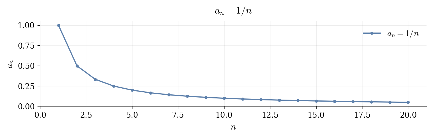
- Let a_n = 1/n. Then (a_n) = \{1, 1/2, 1/3, 1/4, \dots\}. As n increases, a_n approaches zero.
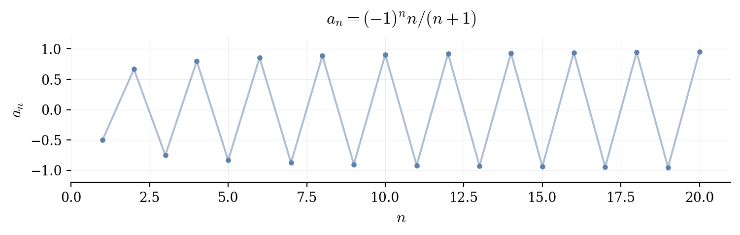
- Consider a_n = (-1)^n \cdot \frac{n}{1+n}, which produces \left\{-\frac{1}{2}, \frac{2}{3}, -\frac{3}{4}, \frac{4}{5}, -\frac{5}{6}, \dots\right\}. This sequence diverges: terms with even n approach +1, while those with odd n approach -1. The sequence oscillates indefinitely without settling to a single value.
- A patient’s systolic blood pressure, measured weekly over several months, might exhibit the pattern shown below. Here the sequence reflects a real process: the patient’s cardiovascular response to treatment.
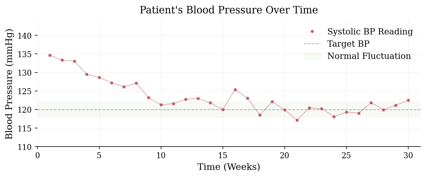
The first two examples are entirely abstract; the third reminds us that sequences often encode empirical observations. In each case, we study the same mathematical object—a function from \mathbb{N} to \mathbb{R}—but the interpretations differ.
2.3 Recursive Sequences
So far, we’ve defined sequences by giving an explicit formula: a_n = 1/n, or a_n = (-1)^n. But many natural processes don’t work this way. Population growth, compound interest, iterative algorithms—in these settings, each step depends on the previous one. We don’t know the n-th term directly; we know how to get from one term to the next. This leads to a different way of specifying sequences.
As we’ve seen in many applications, the next term in the sequence depends on the previous term(s). Such sequences are called recursive.
Even with simple rules, recursive sequences can display diverse behaviors: convergence, divergence, monotone growth, or very rapid escalation. Studying these sequences builds intuition for limits, series, and the stepwise evolution of functions.
Definition 2.2 (Recursive Sequence) A sequence (a_n) is recursive if there exists a function f : \mathbb{R} \to \mathbb{R} and an initial value a_0 \in \mathbb{R} such that
a_{n+1} = f(a_n, a_{n-1},\ldots), \quad n \ge 0.
The function f determines the evolution of the sequence from the initial term.
2.3.0.1 Geometric Recursive Sequence
A geometric sequence is a recursive sequence in which each term is obtained by multiplying the previous term by a fixed number r \in \mathbb{R}. Formally, let (a_n) be defined by
a_0 \in \mathbb{R}, \quad a_{n+1} = r \, a_n \quad \text{for } n \ge 0.
The number r is called the common ratio, and a_0 is the initial term.
The first few terms are
a_0, \; a_0 r, \; a_0 r^2, \; a_0 r^3, \dots, \; a_0 r^n.
2.3.0.2 Arithmetic Recursive Sequence
An arithmetic sequence is a recursive sequence in which each term is obtained by adding a fixed number d \in \mathbb{R} to the previous term. Formally, let (a_n) be defined by
a_0 \in \mathbb{R}, \quad a_{n+1} = a_n + d \quad \text{for } n \ge 0.
The number d is called the common difference, and a_0 is the initial term.
The first few terms are
a_0, \; a_0 + d, \; a_0 + 2d, \; a_0 + 3d, \dots, \; a_0 + n d.
2.3.0.3 Heron’s Method for \sqrt{2}
Let (a_n) be defined recursively by
a_0 = 1, \quad a_{n+1} = \frac{1}{2}\left(a_n + \frac{2}{a_n}\right) \quad \text{for } n \ge 0.
This method, historically attributed to Heron of Alexandria (circa 10–70 CE), is an early instance of what is now called the Newton–Raphson method for approximating roots. The sequence (a_n) produced by this recursion is
1, \; 1.5, \; 1.4167, \; 1.4142, \; 1.4142, \dots
Each iteration produces a value closer to \sqrt{2} than the previous one. Although we have not yet introduced limits rigorously, inspection shows that (a_n) converges to a fixed point satisfying x = \frac{1}{2}\left(x + \tfrac{2}{x}\right), i.e., x = \sqrt{2}.
2.3.0.4 Simple Oscillation
a_0 = 1, \quad a_{n+1} = -a_n
The sequence alternates between two values:
1, -1, 1, -1, 1, -1, \dots
Here, the values remain bounded—they do not grow without limit—but they also do not settle near a single number. Instead, the sequence oscillates indefinitely. We conclude that recursive sequences can be bounded yet fail to “stabilize.”
ImportantSequences as Dynamical Systems
Note: The following sections on nonlinear dynamics, chaos, and fractals explore phenomena that extend beyond the standard Calculus 1 curriculum. They are included to illustrate the depth and richness of recursive sequences and to reward readers inclined toward further exploration. Readers not yet comfortable with these concepts may skip them without loss of continuity in the development of fundamental sequence theory.
2.3.1 Linear Recurrences: The Fibonacci Sequence
The Fibonacci sequence is perhaps the most famous recursive sequence there is. The Fibonacci sequence (F_n) is defined recursively by F_0 = 0, \quad F_1 = 1, \quad F_{n+2} = F_{n+1} + F_n \quad \text{for } n \ge 0. Its study can be traced at least as far back as the Liber Abaci (1202) by Fibonacci, who introduced the sequence in the context of a population growth problem for rabbits. More generally, the sequence arises in combinatorial enumerations and in various natural patterns.
To obtain an explicit formula, consider solutions of the form F_n = r^n. Substituting into the recurrence yields r^{n+2} = r^{n+1} + r^n \implies r^2 = r + 1. The characteristic equation r^2 - r - 1 = 0 has roots \phi = \frac{1+\sqrt{5}}{2}, \qquad \hat{\phi} = \frac{1-\sqrt{5}}{2}. The general solution is F_n = A \phi^n + B \hat{\phi}^n, where A,B \in \mathbb{R}. Imposing F_0 = 0 and F_1 = 1 gives F_n = \frac{\phi^n - \hat{\phi}^n}{\sqrt{5}}.
2.3.2 Oscillatory Recurrences
Not all recursive sequences exhibit monotonic growth or decay. Consider a_{n+1} = -\frac{1}{2} a_n + \frac{1}{4}. At each step, the sequence moves toward the equilibrium value L = 1/2, but with alternating sign. The closed form, a_n = \left(-\frac{1}{2}\right)^n \left(a_0 - \frac{1}{2}\right) + \frac{1}{2}, reveals that the oscillations decay exponentially. Such sequences model damped oscillations in physics—think of a pendulum with friction—and transient responses in control systems.
2.3.3 Nonlinear Recurrences and Chaos
Linear recurrences, though transparent in their behavior, fail to illustrate the full complexity of discrete dynamics. Introducing nonlinearity substantially increases analytical difficulty. Consider the logistic map x_{n+1} = r \, x_n (1 - x_n), here x_n = P_n / K, which is called the fraction of capacity. Proposed by R. M. May (1976) as a model for population growth under resource constraints. Here 0 \le x_0 \le 1 denotes the initial population relative to carrying capacity, and r > 0 is the growth parameter.
For small r, the sequence (x_n) converges to a fixed point. As r increases, the fixed point becomes unstable and the sequence exhibits period-doubling: oscillating between two values, then four, then eight, and so on. Beyond r \approx 3.57, (x_n) behaves chaotically: no stable pattern emerges, and arbitrarily small changes in x_0 yield substantially different outcomes.
This sensitive dependence on initial conditions exemplifies deterministic chaos. Despite the absence of randomness, the long-term behavior of (x_n) is effectively unpredictable. The bifurcation diagram below illustrates this transition from order to chaos.
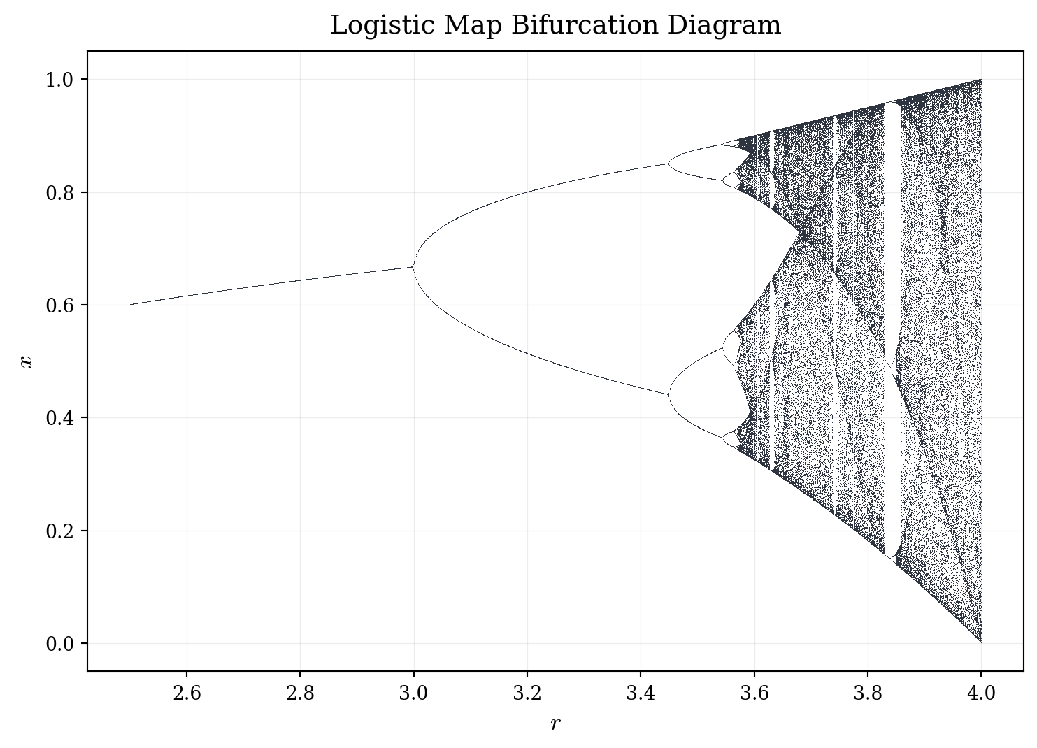
For each fixed r, the vertical slice of the bifurcation diagram shows the long-term behavior of the sequence (x_n) with x_0 = 0.5. If r < 3, the sequence converges to a single fixed point. As r increases, the sequence undergoes successive period-doublings. Beyond the onset of chaos, (x_n) is dense in a Cantor-like set, producing a fractal structure from the quadratic iteration.
The logistic map occurs in models of population dynamics, neural activity, and fluid flow. Its study led to the identification of universal constants governing the period-doubling route to chaos (Feigenbaum, 1970s).
2.3.4 Quadratic Iterations and Fractals
If we allow sequences to take values in the complex plane, even richer structure emerges. Consider the iteration z_{n+1} = z_n^2 + c, \quad c \in \mathbb{C}, starting from z_0 = 0. For a given c, the sequence either escapes to infinity or remains bounded. The set of c values for which (z_n) stays bounded is the Mandelbrot set, one of the most intricate objects in mathematics.
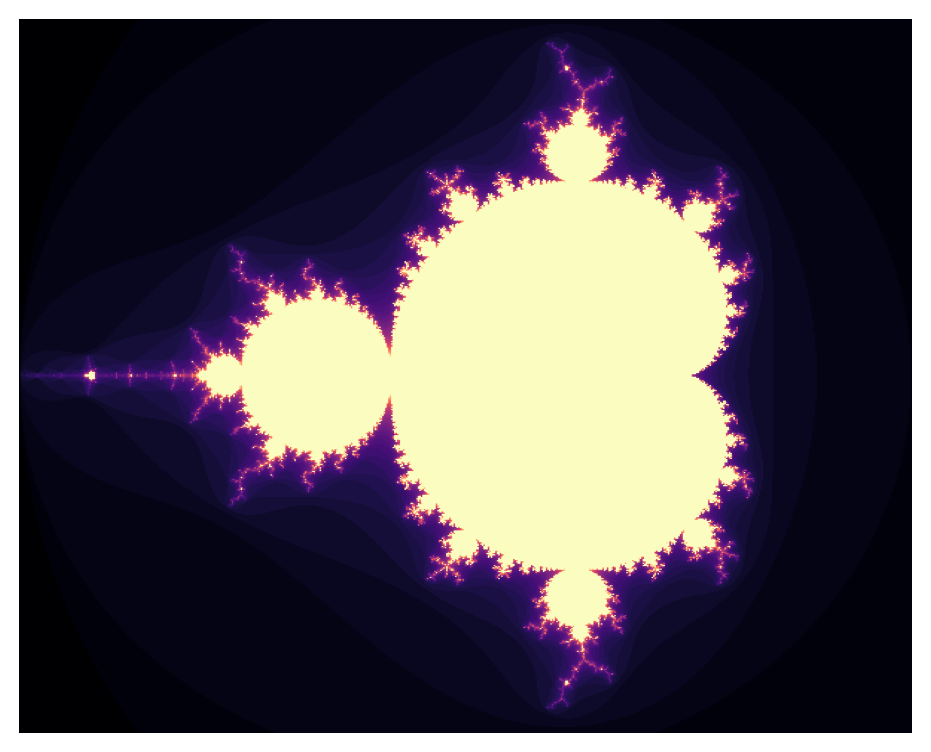
Each pixel corresponds to a complex number c. Dark regions indicate values for which the sequence remains bounded; bright regions escape quickly. The boundary of the Mandelbrot set is infinitely complex: zooming in reveals self-similar structures at all scales. This fractal geometry connects the study of sequences to topology, complex dynamics, and even theoretical physics.
2.3.4.1 Examples
1. Discrete recursive model
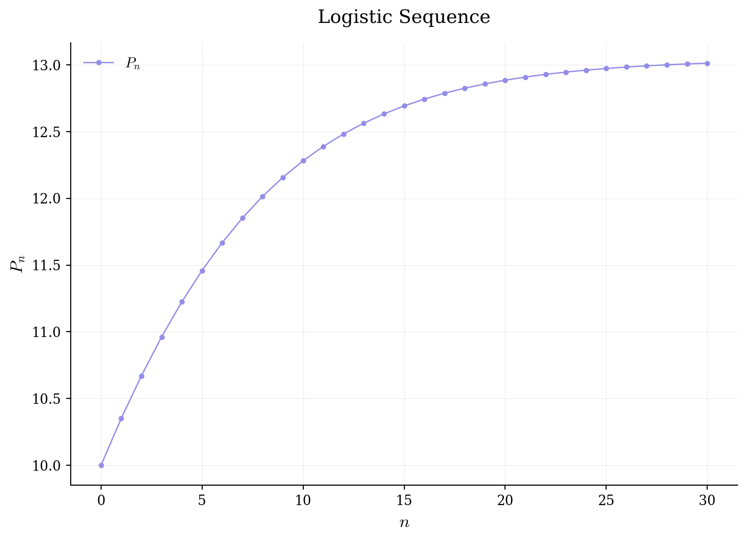
We model a population evolving in discrete generations. Let P_0 be the initial population, and define P_{n+1} = r \, P_n \left(1 - \frac{P_n}{K}\right), where r is the intrinsic growth rate and K the carrying capacity.
This is the discrete logistic equation. Initially, when P_n \ll K, growth is nearly exponential: P_{n+1} \approx r P_n. As P_n approaches K, the factor (1 - P_n/K) suppresses growth, modeling resource limitation. The sequence (P_n) captures the interplay between reproduction and environmental constraints generation by generation.
The continuous analogue is the logistic differential equation, \frac{dP}{dt} = r \, P \left(1 - \frac{P}{K}\right), which we will encounter later. For now, the discrete version suffices to illustrate self-limiting growth.
2. Position of a particle
Suppose we measure the displacement of a vibrating particle at integer times and record \left\{ -\frac{5}{8},\; \frac{17}{32},\; -\frac{65}{128},\; \frac{257}{512}, \ldots \right\}. We seek a closed form for a_n.
Observe the numerators: 5 = 4 + 1, \quad 17 = 16 + 1, \quad 65 = 64 + 1, \quad 257 = 256 + 1. The pattern suggests 4^n + 1. The denominators follow 8 = 2^3, \quad 32 = 2^5, \quad 128 = 2^7, \quad 512 = 2^9, giving 2^{2n+1}. The signs alternate, so a_n = (-1)^n \, \frac{4^n + 1}{2^{2n+1}} = (-1)^n \, \frac{4^n + 1}{2 \cdot 4^n} = (-1)^n \left( \frac{1}{2} + \frac{1}{2 \cdot 4^n} \right).
3. Experimental data
If a_n measures the concentration of a drug in a patient’s bloodstream at successive hours, then (a_n) is the empirical sequence. Analyzing its behavior—whether it decays, stabilizes, or oscillates—informs dosing protocols and pharmacokinetic models.
WarningProblem Set
Let (a_n) be the sequence defined by a_n = \frac{3n-1}{n+2}, \quad n\in\mathbb{N}
Compute a_1, a_2, and a_3.
Write the first four terms of the sequence explicitly as an ordered list.
Show that a_n may be rewritten in the form a_n = 3 - \frac{7}{\,n+2\,}.
Using this expression, explain why the change from a_n to a_{n+1} becomes smaller as n increases.
Consider the recursively defined sequence (b_n) given by b_0 = 1, \qquad b_{n+1} = 2b_n + 1 \quad\text{for } n \ge 0.
Compute b_1, b_2, and b_3.
Guess a closed-form expression for b_n.
Prove that your formula is correct using mathematical induction.
Explain one advantage and one disadvantage of defining a sequence recursively rather than explicitly.
Define a sequence (c_n) by c_n = (-1)^n \frac{n+1}{n+2}.
Write out the first six terms of the sequence.
Separate the sequence into its even-indexed terms and odd-indexed terms.
Describe the pattern of signs in the sequence.
Describe how the magnitudes of the terms change as n increases.
WarningSolutions
Compute directly from the definition a_n = \frac{3n-1}{n+2}. Thus a_1 = \frac{3(1)-1}{1+2} = \frac{2}{3},\qquad a_2 = \frac{6-1}{4} = \frac{5}{4},\qquad a_3 = \frac{9-1}{5} = \frac{8}{5}.
The first four terms are \frac{2}{3},\; \frac{5}{4},\; \frac{8}{5},\; \frac{11}{6}.
We rewrite a_n by separating the numerator: \frac{3n-1}{n+2} = \frac{3(n+2)-7}{n+2} = 3 - \frac{7}{n+2}.
From a_n = 3 - \dfrac{7}{n+2} the only n-dependent part is the fraction 7/(n+2). As n increases the denominator grows and the fraction decreases in magnitude. Moreover, a_{n+1}-a_n = 7\left(\frac{1}{n+2}-\frac{1}{n+3}\right)=\frac{7}{(n+2)(n+3)}, which tends to 0 as n\to\infty. Hence the change between successive terms becomes smaller as n increases.
Using the recursion, b_1 = 2b_0 + 1 = 3,\qquad b_2 = 2b_1 + 1 = 7,\qquad b_3 = 2b_2 + 1 = 15.
From the values 1,3,7,15,\dots we observe each term is one less than a power of 2. This suggests b_n = 2^{n+1}-1.
Proof by induction.
Base case. For n=0, 2^{0+1}-1=2-1=1=b_0, so the formula holds.
Inductive step. Assume b_n=2^{n+1}-1 for some n\ge0. Then b_{n+1}=2b_n+1=2(2^{n+1}-1)+1=2^{n+2}-2+1=2^{n+2}-1, so the formula holds for n+1. By induction the formula is true for all n\ge0. \square
An advantage of recursive definitions: they describe the step-by-step evolution of a process and often mirror how values are generated in applications.
A disadvantage: computing b_n from a purely recursive definition typically requires computing all previous terms, whereas an explicit formula allows direct computation of the n-th term.
The first six terms are \frac{2}{3},\, -\frac{3}{4},\, \frac{4}{5},\, -\frac{5}{6},\, \frac{6}{7},\, -\frac{7}{8}.
For even indices n=2k, c_{2k} = \frac{2k+1}{2k+2}. For odd indices n=2k+1, c_{2k+1} = -\frac{2k+2}{2k+3}.
The factor (-1)^n causes the sign to alternate: positive for even n and negative for odd n.
The magnitudes satisfy |c_n| = \frac{n+1}{n+2}, which increases toward 1 as n increases, though it is always less than 1.
You can download the problem set here: