3 Convergence of Sequences

3.1 Definition and Convergence Properties

This section rigorously defines convergence and establishes the foundational theorems for calculating limits. Recall from the previous section that sequences such as a_n = 1/n, population sizes, particle positions, or experimental measurements can either stabilize, oscillate, or diverge. The definitions here formalize those intuitive ideas.

3.1.1 Measuring Closeness

In order to have a meaningfull discussion of convergence, we first need a way to measure distance between numbers on the real line. Let p, q \in \mathbb{R} be any two real numbers. Their distance is defined by the absolute difference

d(p, q) = |p - q|.

This function d is called a metric on \mathbb{R}. It satisfies the natural properties of distance

Non-negativity: d(p, q) \ge 0, with equality if and only if p = q.
Symmetry: d(p, q) = d(q, p).
Triangle inequality: d(p, r) \le d(p, q) + d(q, r) for any p, q, r \in \mathbb{R}.

Intuitively, d(p, q) tells us how far apart two numbers are on the number line.

Now, consider a sequence \{a_n\} and a proposed limit a. The distance between a term a_n and the limit is given by the same metric

d(a_n, a) = |a_n - a|.

A sequence converges to a if this distance becomes arbitrarily small as n grows large. In other words, the terms eventually “cluster” around a, just like the population or blood pressure measurements approached a target value in our earlier examples.

3.1.2 Formalizing Closeness

To define “arbitrarily close,” we introduce \varepsilon > 0, a tolerance level around the limit a. The condition |a_n - a| < \varepsilon means a_n lies strictly within (a-\varepsilon, a+\varepsilon).

This closeness must hold eventually, quantified by a threshold index N. That is, there exists N such that all n \ge N satisfy |a_n - a| < \varepsilon. This formalizes the idea of a sequence “settling down” from the sequences section.

Definition 3.1 (Convergence) A sequence \{a_n\} converges to a limit a \in \mathbb{R} if for every \varepsilon > 0, there exists N \in \mathbb{N} such that for all n \ge N

|a_n - a| < \varepsilon

We write \lim_{n\to\infty} a_n = a or a_n \to a. If no such a exists, the sequence diverges.

Convergence is a statement about the tail of the sequence, not individual terms. Finitely many terms can be arbitrarily far from the limit; what matters is eventual proximity.

3.1.3 Uniqueness and Boundedness

Theorem 3.1 (Uniqueness of Limits) If a_n \to a and a_n \to a', then a = a'.

Proof.

Assume, for contradiction, that a \neq a'. Set \varepsilon = \tfrac{1}{2} d(a, a') > 0. By definition of convergence, there exist integers N_1 and N_2 such that |a_n - a| < \varepsilon \quad \text{for all } n \ge N_1, and |a_n - a'| < \varepsilon \quad \text{for all } n \ge N_2.

Let N = \max(N_1, N_2). Then for all n \ge N, both inequalities hold simultaneously.

But then, by the triangle inequality, |a - a'| \le |a - a_n| + |a_n - a'| < \varepsilon + \varepsilon = |a - a'|,

a contradiction. Hence, a = a'. \square

Having proved that limits, when they exist, are unique, we can treat convergence as a genuinely well-defined notion. A sequence cannot approach two different points; its eventual behavior is tied to a single value. This fact will serve repeatedly as we analyze further properties of convergent sequences.

The next question is how the individual terms of a convergent sequence behave. If the sequence converges to a fixed number, then the tail of the sequence must remain in a “neighborhood” of that number, and this confinement suggests a global restriction on the size of all terms. This leads naturally to the notion of boundedness.

Definition 3.2 (Bounded Sequence) A sequence \{a_n\} is bounded if there exists M > 0 such that |a_n| \le M for all n \in \mathbb{N}.

The definition of bounded sequences captures the intuitive idea that a sequence doesn’t escape to infinity—its terms stay within some fixed distance from the origin. But what’s the connection to convergence? If a sequence settles down near a limit, it seems plausible that it can’t simultaneously run off to infinity. This intuition is correct.

Theorem 3.2 (Convergent Sequences are Bounded) If a_n \to a, then the sequence \{a_n\} is bounded.

Proof

Take \varepsilon = 1. Since a_n \to a, there exists N such that for all n \ge N, |a_n - a| < 1, implying |a_n| < |a| + 1 for these n.

Define M = \max(|a_1|, |a_2|, \dots, |a_{N-1}|, |a|+1). Then |a_n| \le M for all n, so the sequence is bounded. \square

3.2 Algebra of Limits

Once uniqueness and boundedness are clear, the behavior of limits under algebraic operations almost falls into place.

If two sequences get closer and closer to their respective limits, then adding them term-by-term produces another sequence that gets closer and closer to the sum of those limits. Multiplying them produces a sequence that gets closer and closer to the product. Nothing mysterious is happening—the limiting behavior transfers through the usual arithmetic of real numbers.

The subtle point is that this transfer relies on the control we gained earlier. Without boundedness, for instance, products can misbehave badly. Having the sequence “stay in range” guarantees that the small errors in the tail do not get amplified into something uncontrollable.

The student does not need to memorize these rules. They should feel inevitable: of course the limit of a sum should be the sum of the limits, because the sequences themselves are essentially behaving like their limits near infinity. The formal proofs confirm precisely that intuition.

Theorem 3.3 (Limit Laws) Let (a_n) and (b_n) be convergent sequences with a_n \to a and b_n \to b. Then

a_n \pm b_n \to a \pm b
a_n b_n \to ab
If b_n \neq 0 for all n and b \neq 0, then a_n / b_n \to a / b
If c \in \mathbb{R}, then c a_n \to c a

Proof

Given \varepsilon>0, choose N_1 and N_2 such that for all n \ge N_1, |a_n-a|<\varepsilon/2, and for n \ge N_2, |b_n-b|<\varepsilon/2. Let N = \max(N_1, N_2). Then for all n \ge N |(a_n+b_n) - (a+b)| = |(a_n-a) + (b_n-b)| \le |a_n-a| + |b_n-b| < \varepsilon. Subtraction is entirely analogous. \square
For c \in \mathbb{R}, observe that |c a_n - c a| = |c|\,|a_n - a|. Given \varepsilon>0, choose N such that |a_n - a| < \varepsilon/|c| for n \ge N. Then |c a_n - c a| < \varepsilon. \square
Since b_n \to b, the sequence (b_n) is bounded by Theorem 3.2; say |b_n| \le M for all n. Then |a_n b_n - ab| = |a_n(b_n-b) + b(a_n-a)| \le M |a_n-a| + |b| |b_n-b|. Choosing N large enough ensures both terms are smaller than \varepsilon/2, so their sum is < \varepsilon. \square
Since b_n \to b \neq 0, there exists N_0 such that |b_n| \ge |b|/2 > 0 for all n \ge N_0. Then for n \ge N_0 \left|\frac{a_n}{b_n} - \frac{a}{b}\right| = \frac{|a_n b - a b_n|}{|b_n||b|} = \frac{|(a_n-a)b - a(b_n-b)|}{|b_n||b|} \le \frac{2}{|b|}\left(|b||a_n-a| + |a||b_n-b|\right).
Choosing N large enough that |a_n-a| and |b_n-b| are sufficiently small ensures the quotient converges. \square

Remark: Each step above follows directly from the \varepsilon-N definition of convergence. Working these out carefully is a good exercise in “unpacking” the definition, and it sets the stage for analogous arguments for limits of functions, derivatives, and integrals.

Corollary 3.1 (Powers of Sequences) If a_n \to a and p \in \mathbb{N}, then a_n^p \to a^p.

3.3 Comparison Theorems

Having established algebraic rules for combining limits, we turn to inequalities. If one sequence is always less than another, what can we say about their limits? Intuitively, the ordering should persist in the limit—though we must be careful, as strict inequalities can become weak inequalities at the boundary.

Theorem 3.4 (Comparison Theorem) Let (a_n) and (b_n) be sequences of real numbers satisfying
a_n \le b_n \quad \text{for all } n \in \mathbb{N}. If a_n \to a and b_n \to b, then a \le b.

Proof

Assume, for contradiction, that a > b. Set
\varepsilon = \tfrac{1}{2}(a - b) > 0. Since a_n \to a and b_n \to b, there exist N_1, N_2 \in \mathbb{N} such that for n \ge N_1, |a_n - a| < \varepsilon, and for n \ge N_2, |b_n - b| < \varepsilon. Let N = \max\{N_1, N_2\}. For all n \ge N, a_n > a - \varepsilon = \frac{a + b}{2}, \qquad b_n < b + \varepsilon = \frac{a + b}{2}, so a_n > b_n, contradicting a_n \le b_n for all n. Hence the assumption a > b is impossible, and therefore a \le b. \square

Theorem 3.5 (Squeeze Theorem) If a_n \le b_n \le c_n for all n, and \lim_{n \to \infty} a_n = \lim_{n \to \infty} c_n = a, then \lim_{n \to \infty} b_n = a.

Proof

Let \varepsilon > 0 be given. By definition of the limit, there exist N_1, N_2 \in \mathbb{N} such that n \ge N_1 \implies |a_n - a| < \varepsilon, \qquad n \ge N_2 \implies |c_n - a| < \varepsilon.

Let N = \max(N_1, N_2). Then for all n \ge N, a - \varepsilon < a_n \le b_n \le c_n < a + \varepsilon.

Thus |b_n - a| < \varepsilon, showing that \lim_{n \to \infty} b_n = a. \square

Problem.

Let a_n = \frac{\sin(1/n)}{1/n} for n \in \mathbb{N}. Show that \lim_{n \to \infty} a_n = 1 using Theorem 3.5.

Solution

Let \theta = 1/n for n \in \mathbb{N}. Then \theta > 0 and \theta \to 0 as n \to \infty.

We prove the key inequality \sin \theta < \theta < \tan \theta for 0 < \theta < \frac{\pi}{2} using a geometric argument comparing areas.

The vertical line through A is tangent to the unit circle at A = (1, 0). This line has equation x = 1. The ray from the origin through P has slope \frac{\sin \theta}{\cos \theta}, so its equation is y = x \tan \theta.

Setting x = 1, we get y = \tan \theta. Therefore, the intersection point is T = (1, \tan \theta).

Next, we compare the areas of three regions (all clearly visible in the diagram)

1. Triangle OPA (green):
From basic geometry, we have that the base OA = 1 (along the x-axis) and the height = perpendicular distance from P to the x-axis = \sin \theta

\text{Area}_{OPA} = \frac{1}{2} \cdot \text{base} \cdot \text{height} = \frac{1}{2} \sin \theta

2. Circular sector OPA (blue):
A sector of a circle with radius r and angle \theta (in radians) has area \frac{1}{2} r^2 \theta.

Since r = 1 \text{Area}_{\text{sector}} = \frac{1}{2} \theta

3. Triangle OAT (yellow):
This is a right triangle with base OA = 1 and height AT = \tan \theta (the vertical segment from A to T)

\text{Area}_{OAT} = \frac{1}{2} \tan \theta

By inspection of the diagram, we see that \text{Triangle } OPA \subset \text{Sector} \subset \text{Triangle } OAT

The triangle OPA is entirely contained within the circular sector, which is entirely contained within the larger triangle OAT. Therefore

\frac{1}{2} \sin \theta < \frac{1}{2} \theta < \frac{1}{2} \tan \theta

Multiplying through by 2 \sin \theta < \theta < \tan \theta

Dividing the inequality \sin \theta < \theta < \tan \theta by \sin \theta > 0 (valid for 0 < \theta < \frac{\pi}{2})

1 < \frac{\theta}{\sin \theta} < \frac{\tan \theta}{\sin \theta} = \frac{1}{\cos \theta}

Taking reciprocals (and reversing inequalities) \cos \theta < \frac{\sin \theta}{\theta} < 1

Substituting \theta = 1/n where n \in \mathbb{N} \cos(1/n) < \frac{\sin(1/n)}{1/n} < 1

As n \to \infty, we have 1/n \to 0, so \cos(1/n) \to \cos(0) = 1.

By Theorem 3.5, since both bounds converge to 1 \lim_{n \to \infty} \frac{\sin(1/n)}{1/n} = 1

Therefore, \lim_{n \to \infty} a_n = 1. \square

3.4 Monotone Convergence Theorem

As we have seen, Theorem 3.2 asserts that every convergent sequence is bounded. One might naturally wonder whether the converse holds: do bounded sequences necessarily converge? At first glance, it seems plausible—if the terms of a sequence cannot escape to infinity, one might expect them to settle near some value.

Boundedness alone, however, is not sufficient to guarantee convergence. Consider the sequence a_n = (-1)^n.

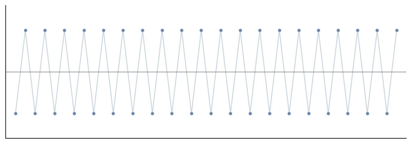
This sequence is clearly bounded between -1 and 1, yet it does not converge, the terms oscillate indefinitely. Thus, while boundedness prevents a sequence from diverging to infinity, it does not ensure that the terms approach a single value.

To get convergence, an additional structural condition is required. The key property is monotonicity, a sequence that is either non-decreasing or non-increasing cannot oscillate. If a monotone sequence is also bounded, these two conditions together constrain the sequence, forcing it to approach a limit. This observation captures the idea behind the Monotone Convergence Theorem.

Definition 3.3 (Monotone Sequence) A sequence {a_n} of real numbers is said to be increasing if a_n \le a_{n+1} for all n \in \mathbb{N}, and strictly increasing if a_n < a_{n+1} for all n. Similarly, {a_n} is decreasing if a_n \ge a_{n+1} for all n, and strictly decreasing if a_n > a_{n+1} for all n. A sequence that is either increasing or decreasing is called monotone.

Intuitively, boundedness provides a ceiling or floor, while monotonicity imposes a directional constraint. Combined, they guarantee convergence.

With this understanding, we are now prepared to state and prove the Monotone Convergence Theorem.

Theorem 3.6 (Monotone Convergence Theorem) Every bounded monotone sequence converges.

Proof

Suppose \{a_n\} is increasing and bounded above. Let \varepsilon>0. Since the sequence is bounded, there exists M with a_n \le M for all n. Choose N such that a_N > M-\varepsilon. Then, for n \ge N, M-\varepsilon < a_N \le a_n \le M, so |a_n - M| < \varepsilon. Hence a_n\to M. The decreasing case is analogous. \square

Note: This proof conveys the main idea, but a fully rigorous argument requires the least upper bound property and the completeness of \mathbb{R}—in particular, these are needed to argue that M=\sup_{n\to\infty}a_n exists and is unique. These concepts are usually developed in a first course in real analysis.

3.4.0.1 Example: Nuclear Reactor

Consider a simplified model of neutron multiplication in a nuclear reactor. When a neutron strikes a fissionable nucleus (such as uranium-235), the nucleus splits, releasing energy and additional neutrons. These new neutrons can then trigger further fission events, creating a chain reaction.

In reality, the behavior of a nuclear reactor involves more complex physics, neutrons have different energy levels, some are absorbed without causing fission, and so on. Our model here is highly idealized, its a thought experiment that captures the essential mathematical structure of multiplicative growth rather than a literal description of the physics.

We model the neutron population using discrete generations. Suppose we observe the system over one unit of time, divided into n equal intervals of length \Delta t = \frac{1}{n}. Let N_k denote the number of neutrons after k generations, with initial “population” N_0 = 1 (in appropriate units).

We adopt the following rule, during each time interval, each neutron present has some probability of causing a fission event that produces additional neutrons. On average, the neutron population increases by a fraction proportional to the current population. Specifically, we assume the population increases by \frac{N_k}{n} at each step.

After the first interval N_1 = N_0 + \frac{N_0}{n} = N_0\left(1 + \frac{1}{n}\right) = 1 + \frac{1}{n}.

After the second interval N_2 = N_1 + \frac{N_1}{n} = N_1\left(1 + \frac{1}{n}\right) = \left(1 + \frac{1}{n}\right)^2.

After k intervals N_k = \left(1 + \frac{1}{n}\right)^k.

After all n intervals a_n = \left(1 + \frac{1}{n}\right)^n.

Proof.

Induct on k \ge 0 to show that a_k = \left(1 + \frac{1}{n}\right)^k.

For k = 0, we have a_0 = 1 = \left(1 + \frac{1}{n}\right)^0. Suppose the statement holds for some k \ge 0. Then

a_{k+1} = a_k \left(1 + \frac{1}{n}\right) = \left(1 + \frac{1}{n}\right)^k \left(1 + \frac{1}{n}\right) = \left(1 + \frac{1}{n}\right)^{k+1}.

And we’re done. \square

As we refine the discretization—taking n larger—we model the chain reaction with finer temporal resolution. Does the sequence \{a_n\} converge?

Physically, we expect the neutron population to remain bounded in this model. Although each generation multiplies the population, the multiplicative factor \left(1 + \frac{1}{n}\right) approaches 1 as n increases. In each interval of length \frac{1}{n}, we add only \frac{1}{n} times the current population—a vanishingly small fraction for large n. The total time is fixed at 1 unit, so the cumulative effect should stabilize. In an actual reactor, control mechanisms and the finite amount of fissionable material would impose physical bounds. Moreover, if the neutron multiplication factor were too large, the reactor would become supercritical and require immediate shutdown—engineers design reactors to operate near criticality, where the population remains controlled.

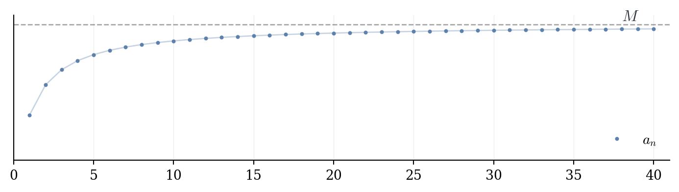
We will make this intuition precise by showing that \{a_n\} is monotone increasing and bounded above, so that Theorem 3.6 applies.

First, we show a_n is increasing. By the binomial theorem, \left(1 + \frac{1}{n}\right)^n = 1 + n \cdot \frac{1}{n} + \binom{n}{2}\frac{1}{n^2} + \binom{n}{3}\frac{1}{n^3} + \cdots + \binom{n}{n}\frac{1}{n^n}.

Each binomial coefficient can be written as \binom{n}{k} = \frac{n(n-1)(n-2)\cdots(n-k+1)}{k!}, so a_n = 1 + 1 + \frac{1}{2!}\left(1 - \frac{1}{n}\right) + \frac{1}{3!}\left(1 - \frac{1}{n}\right)\left(1 - \frac{2}{n}\right) + \cdots

For a_{n+1}, the expansion includes one additional term. Moreover, each factor \left(1 - \frac{k}{n}\right) is replaced by \left(1 - \frac{k}{n+1}\right), which is larger since \frac{k}{n+1} < \frac{k}{n} for k \geq 1. Thus a_{n+1} > a_n.

Next, we show a_n is bounded. From the expansion, each factor \left(1 - \frac{k}{n}\right) \leq 1, so a_n \leq 1 + 1 + \frac{1}{2!} + \frac{1}{3!} + \cdots + \frac{1}{n!}.

Since k! \geq 2^{k-1} for k \geq 1, we have

Proof. k! \geq 2^{k-1}.

We verify k! \geq 2^{k-1} for k \geq 1 by induction. For k = 1, we have 1! = 1 = 2^0. Suppose k! \geq 2^{k-1} for some k \geq 1. Then (k+1)! = (k+1) \cdot k! \geq (k+1) \cdot 2^{k-1} \geq 2 \cdot 2^{k-1} = 2^k, since k+1 \geq 2 for k \geq 1. Thus k! \geq 2^{k-1} for all k \geq 1. \square

a_n \leq 2 + \frac{1}{2} + \frac{1}{4} + \frac{1}{8} + \cdots < 2 + 1 = 3.

By Theorem 3.6, the sequence \{a_n\} converges. We denote this limit by e e = \lim_{n \to \infty} \left(1 + \frac{1}{n}\right)^n.