9 The Fundamental Theorem of Calculus
9.1 The Central Problem
Differentiation extracts instantaneous rates. Given position s(t), we compute velocity v(t) = s'(t). Integration accumulates total change. Given velocity v(t), we compute displacement \int_a^b v(t) \, dt. These operations address opposite questions, yet they are intimately connected. If we differentiate to obtain a rate, then integrate that rate, we should recover the original quantity’s total change. Conversely, if we integrate a function to accumulate area, then differentiate the result, we should recover the original function.
This duality is not a coincidence. The Fundamental Theorem of Calculus establishes that differentiation and integration are inverse operations, linked by the relationship between local and global behavior.
9.1.1 The Accumulation Function
Fix f : [a,b] \to \mathbb{R} integrable. For each x \in [a,b], we can integrate f from a to x:
Definition 9.1 (Accumulation Function) The accumulation function (or integral function) of f with base point a is F(x) = \int_a^x f(t) \, dt, \quad x \in [a,b].
Notation note: We use t as the integration variable to distinguish it from the upper limit x. The variable t is a “dummy variable”—it disappears after integration. The function F depends on x, not on t.
F(x) measures the accumulated contribution of f from a up to x.
If f(t) \geq 0, then F(x) is the area under f from a to x
F(a) = \int_a^a f(t) \, dt = 0 (no accumulation over a point)
As x increases, F(x) accumulates more contribution from f
If f(t) > 0, then F is increasing; if f(t) < 0, then F is decreasing
Example 9.1 (Linear Accumulation) Let f(t) = 2t on [0,3], and define F(x) = \int_0^x 2t \, dt.
For x \in [0,3], partition [0,x] into n equal subintervals. Since f is increasing, using right endpoints: F(x) = \lim_{n \to \infty} \sum_{i=1}^n 2\left(\frac{ix}{n}\right) \cdot \frac{x}{n} = \lim_{n \to \infty} \frac{2x^2}{n^2} \sum_{i=1}^n i = \lim_{n \to \infty} \frac{2x^2}{n^2} \cdot \frac{n(n+1)}{2} = x^2.
So F(x) = x^2. Notice: F'(x) = 2x = f(x).
The derivative of the accumulation function gives back the original function. This is no accident.
9.2 The First Fundamental Theorem
The accumulation function F(x) = \int_a^x f(t) \, dt converts an integrable function f into a new function F. What are the properties of F?
Theorem 9.1 (First Fundamental Theorem of Calculus) Let f : [a,b] \to \mathbb{R} be integrable. Define F(x) = \int_a^x f(t) \, dt, \quad x \in [a,b].
Then:
- F is continuous on [a,b]
- If f is continuous at c \in [a,b], then F is differentiable at c and F'(c) = f(c).
Accumulating the rate f gives a quantity F whose instantaneous rate of change is f. The derivative undoes the integral.
Theorem 9.1 says that integration produces antiderivatives \frac{d}{dx} \int_a^x f(t) \, dt = f(x).
This is one half of the inverse relationship.
TipProof.
Continuity of F.
Let x, x+h \in [a,b]. By additivity of the integral (Theorem 8.6), F(x+h) - F(x) = \int_a^{x+h} f(t) \, dt - \int_a^x f(t) \, dt = \int_x^{x+h} f(t) \, dt.
Since f is integrable on [a,b], it is bounded: there exists M > 0 with |f(t)| \leq M for all t \in [a,b]. Thus |F(x+h) - F(x)| = \left|\int_x^{x+h} f(t) \, dt\right| \leq \int_x^{x+h} |f(t)| \, dt \leq M|h|.
Given \varepsilon > 0, choose \delta = \varepsilon/M. Then |h| < \delta implies |F(x+h) - F(x)| < \varepsilon. Thus F is continuous at x.
Differentiability when f is continuous.
Assume f is continuous at c. We must show \lim_{h \to 0} \frac{F(c+h) - F(c)}{h} = f(c).
From Part 1, \frac{F(c+h) - F(c)}{h} = \frac{1}{h} \int_c^{c+h} f(t) \, dt.
Since f is continuous at c, given \varepsilon > 0, there exists \delta > 0 such that |t - c| < \delta implies |f(t) - f(c)| < \varepsilon.
For |h| < \delta, every t \in [c, c+h] (or [c+h, c] if h < 0) satisfies |t - c| < \delta, so f(c) - \varepsilon < f(t) < f(c) + \varepsilon.
Integrating from c to c+h (and noting the integral reverses sign if h < 0): (f(c) - \varepsilon)h < \int_c^{c+h} f(t) \, dt < (f(c) + \varepsilon)h \quad \text{if } h > 0, (f(c) + \varepsilon)h < \int_c^{c+h} f(t) \, dt < (f(c) - \varepsilon)h \quad \text{if } h < 0.
In both cases, dividing by h gives \left|\frac{1}{h}\int_c^{c+h} f(t) \, dt - f(c)\right| < \varepsilon.
Thus \lim_{h \to 0} \frac{F(c+h) - F(c)}{h} = f(c). \quad \square
Corollary 9.1 (Existence of Antiderivatives) If f is continuous on [a,b], then F(x) = \int_a^x f(t) \, dt is an antiderivative of f: F'(x) = f(x) for all x \in [a,b].
Remark on discontinuities. Theorem 9.1 requires f continuous at c for F'(c) = f(c) to hold. If f has a jump discontinuity at c, then F may not be differentiable at c, or the derivative may not equal f(c).
Example 9.2 (Accumulation with Discontinuity) Let f(t) = \begin{cases} 0 & t < 1 \\ 1 & t \geq 1 \end{cases} on [0,2]. Then,
F(x) = \int_0^x f(t) \, dt = \begin{cases} 0 & x < 1 \\ x - 1 & x \geq 1 \end{cases}.
At x = 1:
Left derivative: \lim_{h \to 0^-} \frac{F(1+h) - F(1)}{h} = \lim_{h \to 0^-} \frac{0 - 0}{h} = 0
Right derivative: \lim_{h \to 0^+} \frac{F(1+h) - F(1)}{h} = \lim_{h \to 0^+} \frac{h}{h} = 1
The derivatives don’t match, so F is not differentiable at x=1. But F is continuous everywhere—integration “smooths out” jump discontinuities.
9.2.1 Differentiating Integrals with Variable Limits
The First Fundamental Theorem treats integrals of the form F(x) = \int_a^x f(t)\,dt. In many situations, the limits of integration depend on x. The following result extends Theorem 9.1 to this setting.
Theorem 9.2 (Leibniz Rule) Let f be continuous on an interval containing the values of \alpha(x) and \beta(x), where \alpha and \beta are differentiable. Define G(x) = \int_{\alpha(x)}^{\beta(x)} f(t)\,dt. Then G is differentiable and G'(x) = f(\beta(x))\,\beta'(x) - f(\alpha(x))\,\alpha'(x).
TipProof.
By additivity of the integral, \int_{\alpha(x)}^{\beta(x)} f(t)\,dt = \int_a^{\beta(x)} f(t)\,dt - \int_a^{\alpha(x)} f(t)\,dt for any fixed a. By Theorem 9.1 and the chain rule, \frac{d}{dx}\int_a^{\beta(x)} f(t)\,dt = f(\beta(x))\beta'(x), \frac{d}{dx}\int_a^{\alpha(x)} f(t)\,dt = f(\alpha(x))\alpha'(x).
Subtracting yields the formula. \square
9.2.2 Antiderivatives and Indefinite Integrals
Theorem 9.1 guarantees that continuous functions have antiderivatives. But antiderivatives are not unique.
Definition 9.2 (Antiderivative) A function F is an antiderivative of f on [a,b] if F'(x) = f(x) for all x \in [a,b].
If F is an antiderivative of f, then so is F + C for any constant C, since (F+C)' = F' = f.
Theorem 9.3 (Antiderivatives Differ by Constants) If F and G are both antiderivatives of f on [a,b], then F - G is constant on [a,b].
TipProof.
Let H = F - G. Then H'(x) = F'(x) - G'(x) = f(x) - f(x) = 0 for all x \in [a,b].
By the Mean Value Theorem, if H' = 0 everywhere, then H is constant. \square
Notation. We denote the family of all antiderivatives of f by \int f(x) \, dx = F(x) + C, where F is any particular antiderivative and C is an arbitrary constant. This is called the indefinite integral or general antiderivative of f.
The indefinite integral \int f(x) \, dx represents a family of functions, not a number. The definite integral \int_a^b f(x) \, dx is a specific real number.
Examples:
\int x^2 \, dx = \frac{x^3}{3} + C, since \frac{d}{dx}\left(\frac{x^3}{3}\right) = x^2
\int \cos x \, dx = \sin x + C, since \frac{d}{dx}(\sin x) = \cos x
\int e^x \, dx = e^x + C, since \frac{d}{dx}(e^x) = e^x
9.3 The Second Fundamental Theorem
Theorem 9.1 tells us that integration produces antiderivatives. The converse question: if we already have an antiderivative, can we compute the integral directly?
Theorem 9.4 (Second Fundamental Theorem of Calculus) Let f : [a,b] \to \mathbb{R} be integrable, and let F be any antiderivative of f on [a,b] (i.e., F'(x) = f(x) for all x \in [a,b]). Then \int_a^b f(x) \, dx = F(b) - F(a).
Notation: We write F(b) - F(a) = \left[F(x)\right]_a^b or F(x) \Big|_a^b.
To compute the integral of f, find any antiderivative F and evaluate it at the endpoints. The definite integral equals the net change in F over [a,b].
This is the computational payoff: instead of computing limits of Riemann sums, we perform two function evaluations.
TipProof.
By Theorem 9.1, the accumulation function G(x) = \int_a^x f(t) \, dt satisfies G'(x) = f(x) (assuming f continuous; the general case requires more care).
Since F is also an antiderivative of f, by Theorem 9.3, there exists a constant C such that F(x) = G(x) + C \quad \text{for all } x \in [a,b].
Evaluating at x = a: F(a) = G(a) + C = \int_a^a f(t) \, dt + C = 0 + C = C.
Thus C = F(a), so G(x) = F(x) - F(a).
Evaluating at x = b: G(b) = F(b) - F(a).
But G(b) = \int_a^b f(t) \, dt by definition, so \int_a^b f(x) \, dx = F(b) - F(a). \quad \square
If f(x) \geq 0, then F(x) = \int_a^x f(t) \, dt is the area function. The total area from a to b is F(b) - F(a)—the net increase in the area function.
9.3.1 Computing Integrals via Antiderivatives
Theorem 9.4 transforms integration into an algebraic problem: find an antiderivative, evaluate at endpoints.
Example 9.3 (Integrating a Quadratic) Compute \int_0^1 x^2 \, dx.
An antiderivative of f(x) = x^2 is F(x) = \frac{x^3}{3} (since F'(x) = x^2). By Theorem 9.4: \int_0^1 x^2 \, dx = \left[\frac{x^3}{3}\right]_0^1 = \frac{1^3}{3} - \frac{0^3}{3} = \frac{1}{3}.
This confirms our earlier computation via Riemann sums, but with far less work.
Example 9.4 (Integrating Sine) Compute \int_0^{\pi} \sin x \, dx.
An antiderivative of \sin x is F(x) = -\cos x. Thus: \int_0^{\pi} \sin x \, dx = [-\cos x]_0^{\pi} = (-\cos \pi) - (-\cos 0) = -(-1) - (-1) = 1 + 1 = 2.
Example 9.5 (Integrating Reciprocal) Compute \int_1^e \frac{1}{x} \, dx.
An antiderivative of \frac{1}{x} is \ln x (for x > 0). Thus: \int_1^e \frac{1}{x} \, dx = [\ln x]_1^e = \ln e - \ln 1 = 1 - 0 = 1.
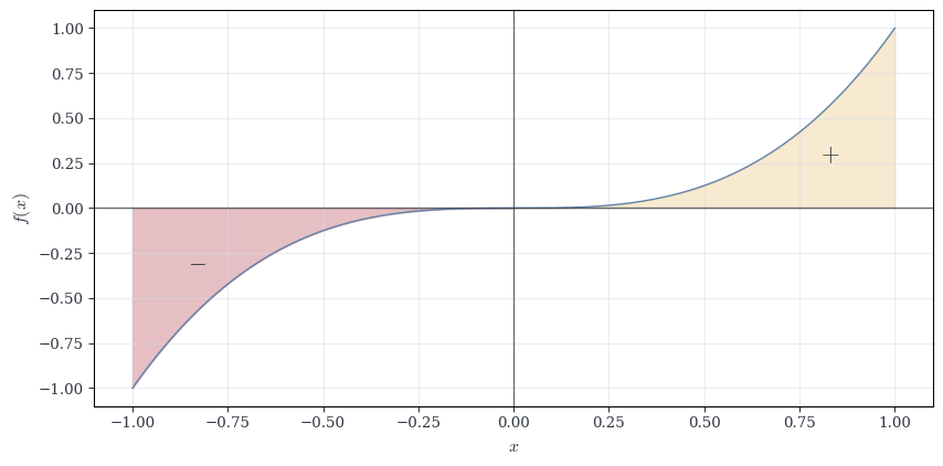
Example 9.6 (Integrating an Odd Function) Compute \int_{-1}^1 x^3 \, dx.
An antiderivative of x^3 is \frac{x^4}{4}. Thus: \int_{-1}^1 x^3 \, dx = \left[\frac{x^4}{4}\right]_{-1}^1 = \frac{1^4}{4} - \frac{(-1)^4}{4} = \frac{1}{4} - \frac{1}{4} = 0.
This makes sense geometrically: x^3 is an odd function, so the area above the x-axis on [0,1] cancels the area below on [-1,0].
9.4 Applications & Extensions
9.4.1 The Net Change Theorem
Theorem 9.4 has a useful interpretation in terms of rates and accumulation.
Theorem 9.5 (Net Change Theorem) If f = F' is the rate of change of F, then \int_a^b f(x) \, dx = F(b) - F(a) is the net change in F over [a,b].
This formalizes our opening intuition: if you know the instantaneous rate at every moment, integrate to get total change.
Applications:
Velocity and displacement. If v(t) is velocity at time t, then \int_{t_0}^{t_1} v(t) \, dt = s(t_1) - s(t_0) is the net displacement (change in position).
Marginal cost. If C'(x) is the marginal cost to produce x units, then \int_{x_1}^{x_2} C'(x) \, dx = C(x_2) - C(x_1) is the total cost to increase production from x_1 to x_2 units.
Population growth. If P'(t) is the rate of population change, then \int_{t_0}^{t_1} P'(t) \, dt = P(t_1) - P(t_0) is the net population change.
Example 9.7 (Velocity and Net Displacement) A particle moves along a line with velocity v(t) = 3t^2 - 6t + 2 m/s for t \in [0,3] seconds. What is the net displacement?
The position function s(t) satisfies s'(t) = v(t), so: \text{Net displacement} = \int_0^3 (3t^2 - 6t + 2) \, dt = \left[t^3 - 3t^2 + 2t\right]_0^3.
Evaluating: = (3^3 - 3 \cdot 3^2 + 2 \cdot 3) - (0) = 27 - 27 + 6 = 6 \text{ meters}.
The particle ends up 6 meters from its starting position.
9.4.2 Signed Area and Absolute Area
The definite integral \int_a^b f(x) \, dx computes signed area: regions above the x-axis contribute positively, regions below contribute negatively.
If f changes sign on [a,b], the integral gives the net area (positive area minus negative area), not the total area enclosed.
Example 9.8 (Signed Area for Sine) Consider f(x) = \sin x on [0, 2\pi].
\int_0^{2\pi} \sin x \, dx = [-\cos x]_0^{2\pi} = (-\cos 2\pi) - (-\cos 0) = -1 - (-1) = 0.
But the graph of \sin x encloses area—it’s positive on [0,\pi] and negative on [\pi, 2\pi]. The areas cancel.
To find the total area (without regard to sign), integrate |f(x)|: \text{Total area} = \int_a^b |f(x)| \, dx.
For \sin x on [0, 2\pi]:
\int_0^{2\pi} |\sin x| \, dx = \int_0^{\pi} \sin x \, dx + \int_{\pi}^{2\pi} (-\sin x) \, dx.
Computing each piece: \int_0^{\pi} \sin x \, dx = [-\cos x]_0^{\pi} = -(-1) - (-1) = 2,
\int_{\pi}^{2\pi} (-\sin x) \, dx = [\cos x]_{\pi}^{2\pi} = 1 - (-1) = 2.
Total area: 2 + 2 = 4.
General principle: If f changes sign at points c_1, c_2, \ldots, c_k in [a,b], then \int_a^b |f(x)| \, dx = \sum_{i} \left|\int_{c_{i-1}}^{c_i} f(x) \, dx\right|,
where we integrate over each interval where f maintains constant sign and sum the absolute values.
9.4.3 Symmetry: Even and Odd Functions
Symmetry often allows definite integrals to be evaluated with minimal computation.
Definition 9.3 (Even and Odd Functions) A function f is even if f(-x)=f(x) for all x.
A function f is odd if f(-x)=-f(x) for all x.
Theorem 9.6 (Integrals of Even and Odd Functions) Let f be integrable on [-a,a].
If f is odd, then \int_{-a}^{a} f(x)\,dx = 0.
If f is even, then \int_{-a}^{a} f(x)\,dx = 2\int_0^{a} f(x)\,dx.
TipProof.
Using the substitution x=-u, \int_{-a}^{a} f(x)\,dx = \int_{a}^{-a} f(-u)(-du) = \int_{-a}^{a} f(-u)\,du.
If f is odd, then f(-u)=-f(u), so the integral equals its negative and must be zero.
If f is even, then f(-u)=f(u), and splitting the interval gives \int_{-a}^{a} f(x)\,dx = 2\int_0^{a} f(x)\,dx. \square
9.4.4 Periodic Functions and Integrals
Many functions repeat their behavior over fixed intervals.
Definition 9.4 (Periodic Function) A function f is periodic with period T>0 if f(x+T)=f(x) for all x.
Theorem 9.7 (Integrals of Periodic Functions) If f is integrable and has period T, then \int_a^{a+T} f(x)\,dx is independent of a.
Moreover, for any integer n, \int_a^{a+nT} f(x)\,dx = n\int_0^{T} f(x)\,dx.
TipProof.
Using the substitution u=x-a, \int_a^{a+T} f(x)\,dx = \int_0^T f(u+a)\,du.
By periodicity, f(u+a)=f(u), so the value depends only on one period.
Additivity of the integral yields the second formula. \square
Periodic integrals reduce global behavior to a single fundamental interval.
9.5 The Inverse Relationship: A Structural Perspective
Let’s make the duality between differentiation and integration explicit.
Define the differentiation operator D : C^1([a,b]) \to C([a,b]) by D(F) = F'.
This maps differentiable functions to continuous functions.
Define the integration operator I : C([a,b]) \to C([a,b]) by I(f)(x) = \int_a^x f(t) \, dt.
This maps continuous functions to continuous functions (and in fact, to differentiable functions).
Theorem 9.1 says: D(I(f)) = f. That is, D \circ I = \text{id} on C([a,b]).
Theorem 9.4 says: If F' = f, then I(f)(b) - I(f)(a) = F(b) - F(a). Modulo constants, I(D(F)) = F. That is, I \circ D = \text{id} (up to constants).
The operators are inverse to each other:
Differentiation extracts rates → Integration accumulates
Integration accumulates → Differentiation extracts rates
This is the organizing principle of calculus: local and global perspectives are dual.
| Differentiation | Integration |
|---|---|
| D : F \mapsto F' | I : f \mapsto \int_a^x f(t) \, dt |
| Local (rate at a point) | Global (accumulation over interval) |
| D(I(f)) = f | I(D(F)) = F + C |
| Sensitive to small changes | Robust to isolated discontinuities |
| Linear: D(F+G) = DF + DG | Linear: I(f+g) = If + Ig |
The Fundamental Theorem unifies differential and integral calculus. They are not separate theories—they are two aspects of the same structure.
9.5.1 When Antiderivatives Don’t Have Closed Forms
Theorem 9.4 is powerful, but only when we can find an antiderivative in closed form. Many functions don’t have elementary antiderivatives.
Examples of functions with no elementary antiderivative:
f(x) = e^{-x^2} (the Gaussian)
f(x) = \frac{\sin x}{x} (the sinc function)
f(x) = \frac{1}{\ln x}
These functions are perfectly integrable—\int_a^b e^{-x^2} \, dx exists as a number. But we cannot express the antiderivative using polynomials, exponentials, logarithms, trigonometric functions, and their compositions.
In such cases, we must:
Use numerical methods (Riemann sums, Simpson’s rule, etc.)
Define new functions via integration (e.g., \text{erf}(x) = \frac{2}{\sqrt{\pi}} \int_0^x e^{-t^2} \, dt)
Use series expansions (power series, Taylor series, which we will see in the coming chapter)
The fundamental theorem tells us integrals exist and connects them to antiderivatives. It doesn’t guarantee we can write them in closed form.
9.6 The Mean Value Theorem for Integrals
As a final application, we prove an integral analogue of the Mean Value Theorem for derivatives.
Theorem 9.8 (Mean Value Theorem for Integrals) If f : [a,b] \to \mathbb{R} is continuous, there exists \xi \in [a,b] such that \int_a^b f(x) \, dx = f(\xi)(b-a).
That is, there exists a height f(\xi) such that the rectangle with base [a,b] and height f(\xi) has the same area as the region under f.
TipProof.
Since f is continuous on [a,b], it attains its minimum m and maximum M on this interval (Extreme Value Theorem from Calculus I).
By order preservation (Theorem 8.5), m(b-a) \leq \int_a^b f(x)\,dx \leq M(b-a).
Dividing by b-a > 0: m \leq \frac{1}{b-a}\int_a^b f(x)\,dx \leq M.
By the Intermediate Value Theorem (Calculus I), since f is continuous and takes values m and M, it takes every value in between. Thus there exists \xi \in [a,b] with f(\xi) = \frac{1}{b-a}\int_a^b f(x)\,dx, which rearranges to \int_a^b f = f(\xi)(b-a). \square
WarningProblem Set
The accumulation function and its properties.
Let f(t) = 3t^2 - 2t on [0,2]. Define F(x) = \int_0^x f(t) \, dt. Using the Riemann sum approach from Example 9.1 (partition [0,x] into n equal subintervals and take the limit), compute F(x) explicitly. Verify that F'(x) = f(x).
Now consider g(t) = \begin{cases} t & \text{if } 0 \leq t < 1 \\ 2-t & \text{if } 1 \leq t \leq 2 \end{cases} on [0,2]. Define G(x) = \int_0^x g(t) \, dt. Compute G(x) by splitting the integral at the corner point t=1 (where g is continuous but not differentiable). Show that G is continuous on [0,2] but determine whether G is differentiable at x=1. Explain your answer in terms of Theorem 9.1.
For the function F from part (a), use Theorem 9.4 to compute \int_0^2 (3t^2 - 2t) \, dt directly. Compare this with the value F(2) you computed via Riemann sums. What does this comparison illustrate about the relationship between the two fundamental theorems?
Leibniz rule and differentiation under the integral.
Let G(x) = \int_x^{x^2} (2t+1) \, dt. First, express this integral in terms of accumulation functions: write G(x) = \int_a^{x^2} (2t+1) \, dt - \int_a^x (2t+1) \, dt for any fixed a. Then use Theorem 9.2 to compute G'(x).
Verify your answer from part (a) by first evaluating the integral G(x) = \int_x^{x^2} (2t+1) \, dt explicitly (find an antiderivative of 2t+1 and apply Theorem 9.4), then differentiate the resulting expression directly. Show that both methods yield the same result.
Consider H(x) = \int_{\sin x}^{x^2} t^2 \, dt for x > 0. Use Theorem 9.2 to find H'(x). Explain why the chain rule plays a crucial role in applying the Leibniz rule when the limits of integration are not simply x itself.
Symmetry, periodicity, and the structure of definite integrals.
Compute \int_{-\pi/2}^{\pi/2} (\sin^3 x + x^2 \cos x) \, dx without finding any antiderivatives. Instead, decompose the integrand into even and odd parts and apply Theorem 9.6. Show all steps of your reasoning.
Let f(x) = |\sin x|. Show that f is periodic with period \pi, then use Theorem 9.7 to compute \int_0^{3\pi} |\sin x| \, dx by first computing \int_0^{\pi} |\sin x| \, dx. (Hint: On [0,\pi], we have \sin x \geq 0, so |\sin x| = \sin x.)
Prove that if f is continuous and even on [-a,a], and g is continuous and odd on [-a,a], then \int_{-a}^a f(x)g(x) \, dx = 0. (Hint: Show that the product of an even function and an odd function is odd, then apply Theorem 9.6.)
WarningSolutions
The accumulation function and its properties.
Computing F(x) via Riemann sums. Partition [0,x] into n equal subintervals with t_i = ix/n for i = 0, 1, \ldots, n. The width of each subinterval is \Delta t = x/n.
Since f(t) = 3t^2 - 2t is increasing on [0,x] for x \leq 2/3 (where f'(t) = 6t - 2 \geq 0), we use right endpoints for the Riemann sum: \begin{align*} F(x) &= \lim_{n \to \infty} \sum_{i=1}^n f(t_i) \Delta t \\ &= \lim_{n \to \infty} \sum_{i=1}^n \left[3\left(\frac{ix}{n}\right)^2 - 2\left(\frac{ix}{n}\right)\right] \cdot \frac{x}{n} \\ &= \lim_{n \to \infty} \frac{x}{n} \sum_{i=1}^n \left(\frac{3i^2x^2}{n^2} - \frac{2ix}{n}\right) \\ &= \lim_{n \to \infty} \left[\frac{3x^3}{n^3}\sum_{i=1}^n i^2 - \frac{2x^2}{n^2}\sum_{i=1}^n i\right]. \end{align*}
Using \sum_{i=1}^n i^2 = \frac{n(n+1)(2n+1)}{6} and \sum_{i=1}^n i = \frac{n(n+1)}{2}: \begin{align*} F(x) &= \lim_{n \to \infty} \left[\frac{3x^3}{n^3} \cdot \frac{n(n+1)(2n+1)}{6} - \frac{2x^2}{n^2} \cdot \frac{n(n+1)}{2}\right] \\ &= \lim_{n \to \infty} \left[\frac{x^3(n+1)(2n+1)}{2n^2} - \frac{x^2(n+1)}{n}\right] \\ &= \lim_{n \to \infty} \left[\frac{x^3(2n^2 + 3n + 1)}{2n^2} - \frac{x^2(n+1)}{n}\right] \\ &= x^3 - x^2. \end{align*}
To verify F'(x) = f(x): F'(x) = \frac{d}{dx}(x^3 - x^2) = 3x^2 - 2x = f(x). \quad \square
Computing G(x) with discontinuity. For x \in [0,1], since g(t) = t on this interval: G(x) = \int_0^x t \, dt = \left[\frac{t^2}{2}\right]_0^x = \frac{x^2}{2}.
For x \in [1,2], we split at t=1: \begin{align*} G(x) &= \int_0^1 t \, dt + \int_1^x (2-t) \, dt \\ &= \frac{1}{2} + \left[2t - \frac{t^2}{2}\right]_1^x \\ &= \frac{1}{2} + \left[\left(2x - \frac{x^2}{2}\right) - \left(2 - \frac{1}{2}\right)\right] \\ &= \frac{1}{2} + 2x - \frac{x^2}{2} - \frac{3}{2} \\ &= 2x - \frac{x^2}{2} - 1. \end{align*}
Thus, G(x) = \begin{cases} \frac{x^2}{2} & 0 \leq x < 1 \\ 2x - \frac{x^2}{2} - 1 & 1 \leq x \leq 2 \end{cases}.
Continuity at x=1: \lim_{x \to 1^-} G(x) = \frac{1}{2}, \quad G(1) = 2(1) - \frac{1}{2} - 1 = \frac{1}{2}.
So G is continuous at x=1.
Differentiability at x=1:
Left derivative: \lim_{h \to 0^-} \frac{G(1+h) - G(1)}{h} = \lim_{h \to 0^-} \frac{\frac{(1+h)^2}{2} - \frac{1}{2}}{h} = \lim_{h \to 0^-} \frac{2h + h^2}{2h} = 1.
Right derivative: \lim_{h \to 0^+} \frac{G(1+h) - G(1)}{h} = \lim_{h \to 0^+} \frac{\left[2(1+h) - \frac{(1+h)^2}{2} - 1\right] - \frac{1}{2}}{h} = \lim_{h \to 0^+} \frac{2h - \frac{2h+h^2}{2}}{h} = 1.
Since both one-sided derivatives equal 1, G is differentiable at x=1 with G'(1) = 1 = g(1).
This is consistent with Theorem 9.1: even though g has a corner at t=1, it is continuous there, so G'(1) = g(1). The accumulation function G is actually smoother than g—G is differentiable everywhere while g only has one-sided derivatives at t=1. \square
Comparing Riemann sums with Theorem 9.4. From part (a), F(x) = x^3 - x^2. Thus: F(2) = 2^3 - 2^2 = 8 - 4 = 4.
By Theorem 9.4, since F is an antiderivative of f(t) = 3t^2 - 2t (we verified F'(x) = f(x)): \int_0^2 (3t^2 - 2t) \, dt = F(2) - F(0) = 4 - 0 = 4.
What this illustrates: Theorem 9.1 tells us that the accumulation function F(x) = \int_0^x f(t) \, dt is an antiderivative of f. Theorem 9.4 tells us that to compute a definite integral, we can use any antiderivative and evaluate at endpoints. Here, the accumulation function constructed via Riemann sums is an antiderivative, and when we evaluate it at the endpoints, we get the integral’s value. The two theorems form a complete cycle: integration produces antiderivatives (Theorem 9.1), and antiderivatives compute integrals (Theorem 9.4). \square
Leibniz rule and differentiation under the integral.
Applying Leibniz rule. Choose any fixed a (say a=0). Then: G(x) = \int_x^{x^2} (2t+1) \, dt = \int_0^{x^2} (2t+1) \, dt - \int_0^x (2t+1) \, dt.
By Theorem 9.2, with \alpha(x) = x and \beta(x) = x^2: G'(x) = (2 \cdot x^2 + 1) \cdot 2x - (2 \cdot x + 1) \cdot 1 = (2x^2 + 1)(2x) - (2x + 1).
Simplifying: G'(x) = 4x^3 + 2x - 2x - 1 = 4x^3 - 1. \quad \square
Direct verification. An antiderivative of 2t+1 is t^2 + t. By Theorem 9.4: \begin{align*} G(x) &= \int_x^{x^2} (2t+1) \, dt = [t^2 + t]_x^{x^2} \\ &= [(x^2)^2 + x^2] - [x^2 + x] \\ &= x^4 + x^2 - x^2 - x \\ &= x^4 - x. \end{align*}
Differentiating directly: G'(x) = 4x^3 - 1.
This matches the result from part (a), confirming that Theorem 9.2 gives the correct derivative. The Leibniz rule is powerful because it allows us to differentiate without first evaluating the integral—crucial when antiderivatives are difficult or impossible to express in closed form. \square
Leibniz rule with composition. By Theorem 9.2 with \alpha(x) = \sin x and \beta(x) = x^2: H'(x) = (\beta(x))^2 \cdot \beta'(x) - (\alpha(x))^2 \cdot \alpha'(x) = (x^2)^2 \cdot 2x - (\sin x)^2 \cdot \cos x.
Thus:
H'(x) = 2x^5 - \sin^2 x \cos x.\square
Symmetry, periodicity, and the structure of definite integrals.
Using symmetry to evaluate. Decompose the integrand: \sin^3 x + x^2 \cos x = \underbrace{\sin^3 x}_{\text{odd}} + \underbrace{x^2 \cos x}_{\text{even}}.
It is easy to see that \sin^3(-x) = (\sin(-x))^3 = (-\sin x)^3 = -\sin^3 x, so \sin^3 x is odd.
For x^2 \cos x: (−x)^2 \cos(−x) = x^2 \cos x, so x^2 \cos x is even.
By Theorem 9.6: \int_{-\pi/2}^{\pi/2} \sin^3 x \, dx = 0 \quad \text{(odd function)}.
For the even part: \int_{-\pi/2}^{\pi/2} x^2 \cos x \, dx = 2\int_0^{\pi/2} x^2 \cos x \, dx.
Since we haven’t yet established integration by parts (which would be needed to evaluate \int x^2 \cos x \, dx), we leave this as: \int_{-\pi/2}^{\pi/2} (\sin^3 x + x^2 \cos x) \, dx = 2\int_0^{\pi/2} x^2 \cos x \, dx.
The key point: symmetry reduced the problem to half the interval and eliminated the odd term entirely. \square
Using periodicity. First, verify that f(x) = |\sin x| has period \pi: f(x + \pi) = |\sin(x + \pi)| = |-\sin x| = |\sin x| = f(x).
On [0,\pi], we have \sin x \geq 0, so |\sin x| = \sin x: \int_0^{\pi} |\sin x| \, dx = \int_0^{\pi} \sin x \, dx = [-\cos x]_0^{\pi} = -\cos \pi - (-\cos 0) = -(-1) + 1 = 2.
By Theorem 9.7, since f has period \pi and 3\pi = 3 \cdot \pi: \int_0^{3\pi} |\sin x| \, dx = 3 \int_0^{\pi} |\sin x| \, dx = 3 \cdot 2 = 6. \quad \square
Product of even and odd functions. Let h(x) = f(x)g(x) where f is even and g is odd.
We need to show h is odd: h(-x) = f(-x)g(-x) = f(x) \cdot (-g(x)) = -f(x)g(x) = -h(x).
Since h is odd and continuous (as the product of continuous functions), by Theorem 9.6: \int_{-a}^a f(x)g(x) \, dx = \int_{-a}^a h(x) \, dx = 0.
The product fg satisfies h(-x) = -h(x), so the graph is symmetric with respect to the origin. The area to the left of zero is the negative of the area to the right, so they cancel exactly when integrated over a symmetric interval. This is a powerful computational tool—it allows us to conclude an integral is zero without finding any antiderivative. \square