7 Continuity
7.1 Continuous Functions
We’ve studied how limits describe the behavior of a function near a point. Continuity is the idea that a function behaves nicely at the point—its value actually matches its limit. Formally, f is continuous at a if
\lim_{x \to a} f(x) = f(a).
For instance, f(x) = x^2 is continuous everywhere, and g(x) = \frac{\sin x}{x} can be made continuous at 0 by defining g(0) = 1. On the other hand, h(x) = \frac{1}{x} is not continuous at 0. Continuity captures the difference between functions that “flow smoothly” and those with jumps or breaks.
Several key results help us work with continuous functions, Theorem 7.3 ensures that a continuous function takes on every value between two points on its graph, and Theorem 7.5 guarantees a maximum and minimum on a closed interval. Meanwhile, limit laws for sums, products, and compositions allow us to combine continuous functions without losing continuity.
This chapter introduces the definition of continuity, gives practical examples, and shows how these theorems let us predict function behavior.
7.2 Continuity at a Point
Let f be a function defined on a subset of \mathbb{R}. We want a precise criterion for saying that f is “continuous” at a point.
Definition 7.1 (Continuity at a Point) We say that f is continuous at a point a if for every \varepsilon > 0 there exists \delta > 0 such that |x - a| < \delta \implies |f(x) - f(a)| < \varepsilon.
Note: This is just our definition of convergence from Section 4.3, but we have replaced L with f(a) to ensure that once the function values enter the chosen neighborhood, they remain within it.
Example 7.1 (Continuity of Linear Function) Let f(x) = mx + b and consider the limit as x \to a. We claim
\lim_{x \to a} f(x) = f(a) = ma + b.
Proof
Given \varepsilon > 0, observe
|f(x) - f(a)| = |(mx + b) - (ma + b)| = |m||x - a|.
To make this less than \varepsilon, choose
\delta = \frac{\varepsilon}{|m|} \quad (\text{assuming } m \neq 0).
Then, whenever |x - a| < \delta, we have
|f(x) - f(a)| = |m||x - a| < |m| \delta = \varepsilon. \quad \square
Note: If m = 0, f(x) = b is constant, and any \delta works since |f(x)-f(a)| = 0 < \varepsilon.
Example 7.2 (Continuity of Quadratic Function) Let f(x) = x^2 and consider the limit as x \to 2. We claim
\lim_{x \to 2} f(x) = f(2) = 4.
Proof
Given \varepsilon > 0, observe that
|f(x) - f(2)| = |x^2 - 4| = |x-2||x+2|.
To control this, restrict x to a \delta-neighborhood of 2 such that |x-2| < 1, which ensures x \in (1,3) and |x+2| \le 5. Then
|f(x) - 4| = |x-2||x+2| \le 5 |x-2| < 5 \delta.
Choose \delta = \varepsilon/5. Then whenever |x-2| < \delta, we have
|f(x) - 4| < 5 \delta = \varepsilon. \quad \square
7.3 The Sequential Characterization
The \varepsilon–\delta definition describes continuity directly in terms of neighborhoods: f(x) remains close to f(a) whenever x is sufficiently close to a. Another viewpoint, often better suited for certain arguments, replaces “points near a’’ with sequences that converge to a. A sequence (a_n) with a_n \to a is simply an ordered way of approaching a; if continuity captures stability of the function under small perturbations of the input, then one expects f(a_n) to converge to f(a) whenever (a_n) converges to a.
This expectation is correct, and it leads to an equivalent formulation that frequently simplifies proofs.
Theorem 7.1 (Sequential Formulation of Continuity) Let f be a real-valued function and let a be a point of its domain. Then f is continuous at a exactly when the following holds,
- For every sequence (a_n) with a_n \to a,
- f(a_n) \to f(a).
(\Rightarrow) Assume f is continuous at a. Let (a_n) be any sequence with a_n\to a. Fix \varepsilon>0. By continuity there exists \delta>0 such that
|x-a|<\delta \implies |f(x)-f(a)|<\varepsilon.
Since a_n\to a, there exists N with |a_n-a|<\delta for all n\ge N. For those n the implication above gives |f(a_n)-f(a)|<\varepsilon. As \varepsilon>0 was arbitrary, f(a_n)\to f(a).
(\Leftarrow) Conversely, assume the sequential condition holds and suppose, for contradiction, that f is not continuous at a. Then there exists \varepsilon_0>0 such that for every \delta>0 one can find x with |x-a|<\delta and |f(x)-f(a)|\ge\varepsilon_0. Taking \delta=1/n for each n produces a sequence (a_n) with |a_n-a|<1/n, hence a_n\to a, but |f(a_n)-f(a)|\ge\varepsilon_0 for every n. This prevents f(a_n) from converging to f(a), contradicting the sequential hypothesis. Therefore f must be continuous at a.
This proves the equivalence.
7.4 Continuity on an Interval
Having defined what it means for a function to be continuous at a single point, the next step is to understand how continuity behaves on larger sets. A pointwise definition is essential, but it does not yet capture the global behavior of a function on an entire region. In practice, we rarely study functions at isolated points; instead, we care about how a function acts across an interval such as I=[a,b].
For example, the statements we ultimately want—such as the existence of roots, the guarantee of extrema, and the ability to pass from local information to global conclusions—depend on continuity everywhere on the interval under consideration, not at a single point. Thus the natural question is:
If a function behaves “well’’ at each point of an interval, does this control its behavior on the whole interval?
This leads to the following definition.
Definition 7.2 (Continuity on an Interval) Let I be an interval in \mathbb{R}. A function f is continuous on I if it is continuous at every point a \in I.
Requiring continuity at each point of an interval rules out any sudden jumps, breaks, or singularities. Almost all standard functions—polynomials, exponentials, trigonometric functions—are continuous on every interval they are defined on (their domain), and rational functions are continuous away from points where their denominators vanish.
Examples
- f(x) = x^3 - 2x + 1 is continuous on \mathbb{R}.
- f(x) = \dfrac{x+1}{x^2-4} is continuous on \mathbb{R} \setminus \{-2,2\}.
- \sin x and \cos x are continuous on \mathbb{R}.
Why this matters becomes clear in the next results, Theorem 7.3 ensures that a continuous function on a closed interval cannot avoid intermediate values, and Theorem 7.5 must attain both a maximum and a minimum. These properties rely not on continuity at one point, but on continuity at every point of the interval.
7.5 Algebra of Continuous Functions
Polynomials are continuous, as are linear functions. The question naturally arises: if f and g are continuous at a point, what can be said about f + g, or f \cdot g, or f \circ g?
The answer follows immediately from the limit laws. Since continuity at a is equivalent to \lim_{x \to a} f(x) = f(a), and since limits respect algebraic operations, continuity must likewise be preserved under these operations. The proof amounts to observing that the limit of a sum equals the sum of limits, the limit of a product equals the product of limits, and so forth.
Theorem 7.2 (Algebra of Continuous Functions) Let f and g be continuous at a. Then f \pm g, cf (for any c \in \mathbb{R}), and fg are continuous at a. If additionally g(a) \neq 0, then f/g is continuous at a. If g is continuous at a and f is continuous at g(a), then f \circ g is continuous at a.
The first four statements follow directly from Theorem 5.1. For the sum, observe that \lim_{x \to a} [f(x) + g(x)] = \lim_{x \to a} f(x) + \lim_{x \to a} g(x) = f(a) + g(a), and similarly for the other operations.
For composition, let \varepsilon > 0. Continuity of f at g(a) provides \eta > 0 such that |y - g(a)| < \eta implies |f(y) - f(g(a))| < \varepsilon. Continuity of g at a provides \delta > 0 such that |x - a| < \delta implies |g(x) - g(a)| < \eta. These combine to give that |x - a| < \delta implies |f(g(x)) - f(g(a))| < \varepsilon, establishing continuity of f \circ g at a. \square
Starting from simple building blocks (polynomials, trigonometric functions, exponentials), we can construct more complex continuous functions through algebraic operations and composition. This substantially reduces the burden of verification: rather than returning to the \varepsilon-\delta definition for every new function, we verify continuity by decomposition into known continuous pieces.
Consider rational functions. Any polynomial p(x) = a_n x^n + \cdots + a_0 is continuous on \mathbb{R} because x is continuous (being linear), powers x^n are continuous (by repeated application of the product rule), and finite sums of continuous functions are continuous. A rational function r(x) = p(x)/q(x) is then continuous wherever q(x) \neq 0, by the quotient rule.
The composition rule handles functions like \sin(x^2 + 1) or e^{\sqrt{x}}. If the inner function u(x) is continuous and the outer function v(u) is continuous, then v(u(x)) is continuous wherever both are defined. This extends our repertoire considerably: compositions of polynomials with trigonometric functions, exponentials of rational functions, and so on are all continuous on appropriate domains.
Example 7.3 (Continuity of Composite Functions)
The rational function h(x) = \frac{x^3 - 2x + 5}{x^2 + 1} is continuous on \mathbb{R} because both numerator and denominator are polynomials, and the denominator is never zero. By contrast, f(x) = \frac{\sin x}{x^2 - 4} is continuous only on \mathbb{R} \setminus \{-2, 2\}, where the denominator vanishes.
For g(x) = \sin(x^2 + 1), write g = \sin \circ u where u(x) = x^2 + 1. The polynomial u is continuous everywhere, and \sin is continuous everywhere, so g is continuous on \mathbb{R}.
The function k(x) = \sqrt{\frac{x+1}{x-3}} requires more care. The rational function r(x) = \frac{x+1}{x-3} is continuous where x \neq 3, and the square root is continuous on [0, \infty). Thus k is continuous where both x \neq 3 and r(x) \geq 0. The inequality \frac{x+1}{x-3} \geq 0 holds when the numerator and denominator have the same sign, which occurs on (-\infty, -1] \cup (3, \infty). Therefore k is continuous precisely on this set.
7.5.1 Piecewise Functions
Functions defined piecewise require explicit verification at the points where the definition changes. Consider f(x) = \begin{cases} x^2 & x < 1 \\ 2x - 1 & x \geq 1. \end{cases}
On (-\infty, 1), f coincides with x^2, which is continuous. On (1, \infty), f coincides with 2x - 1, also continuous. The question is whether f is continuous at the transition point x = 1.
We have f(1) = 2(1) - 1 = 1. The left-hand limit is \lim_{x \to 1^-} x^2 = 1, and the right-hand limit is \lim_{x \to 1^+} (2x-1) = 1. Both limits exist and equal f(1), so f is continuous at 1. Hence f is continuous on all of \mathbb{R}.
By contrast, if we modify the definition: g(x) = \begin{cases} x^2 & x < 1 \\ 3 & x = 1 \\ 2x - 1 & x > 1, \end{cases} then g(1) = 3 while \lim_{x \to 1} g(x) = 1. The limit exists but does not equal the function value. This is a removable discontinuity, one that could be eliminated by redefining g(1) = 1. Nevertheless, as defined, g is not continuous at 1.
The general principle is clear: at interior points of each piece, a piecewise function inherits continuity from its component parts. At boundary points, continuity must be verified directly by checking that left and right limits agree with the function value. This is where discontinuities typically appear, if they appear at all.
7.6 The Intermediate Value Theorem
The algebraic properties of continuous functions tell us how to build new continuous functions from old ones. But they don’t reveal deeper consequences of continuity itself. What does it mean, geometrically, for a function to have no jumps? The answer is subtle and profound: a continuous function on an interval cannot skip over values. If it starts below a horizontal line and ends above it, it must cross that line somewhere.
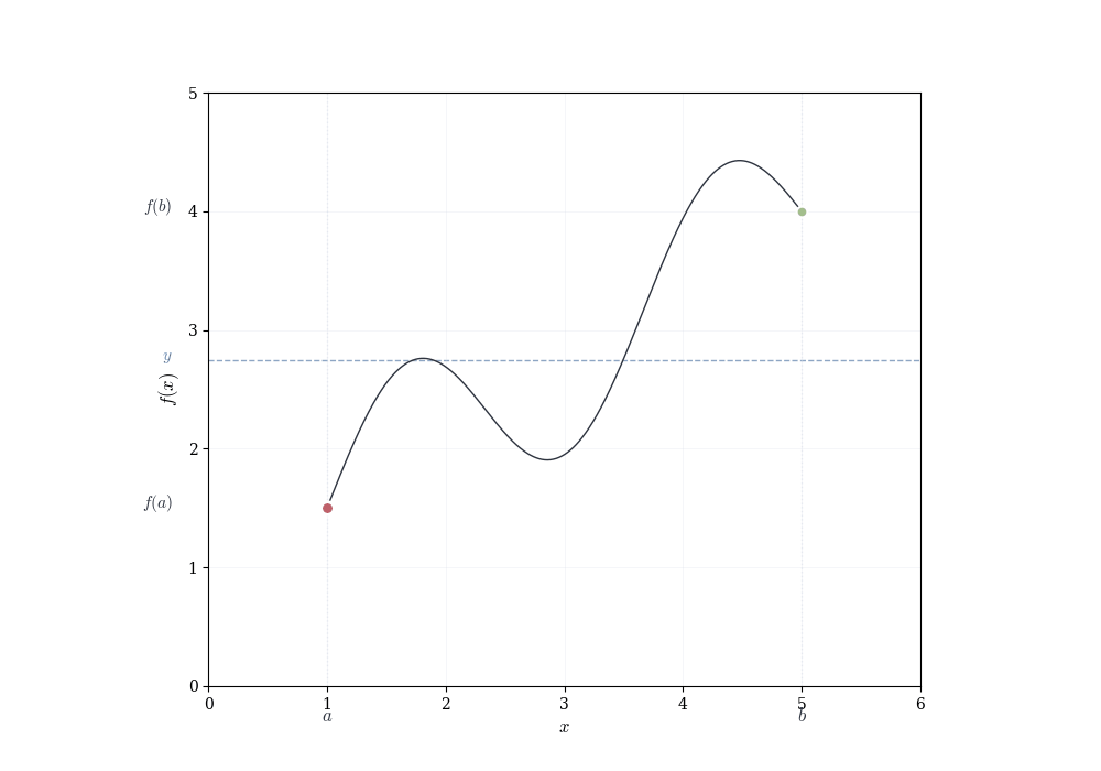
A continuous function on an interval exhibits no jumps or gaps. This elementary observation has consequences: such a function must assume every intermediate value. If f is continuous on [a,b] and f(a) < y < f(b), then there exists some point c between a and b where f(c) = y. The function cannot leap over y without passing through it.
Though this seems obvious from pictures, it is a genuine theorem about the real numbers. Consider f(x) = x^2 - 2 restricted to rational inputs and outputs. We have f(1) = -1 < 0 and f(2) = 2 > 0, so the function changes sign. Yet there is no rational number c where f(c) = 0, because \sqrt{2} is irrational. The intermediate value property fails over \mathbb{Q} precisely because the rationals have gaps. The real numbers fill these gaps and allow the theorem to hold.
Theorem 7.3 (Intermediate Value Theorem) Let f : [a,b] \to \mathbb{R} be continuous. If y lies strictly between f(a) and f(b), then there exists c \in (a,b) such that f(c) = y.
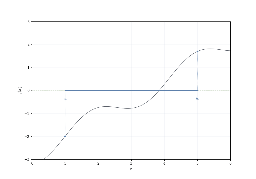
Assume f(a) < y < f(b) (the reverse inequality is handled the same way). The goal is to locate a point c\in[a,b] with f(c)=y by successively halving the interval [a,b].
Set [a_0,b_0]=[a,b] with f(a_0)<y<f(b_0). For n\ge0 let m_n=(a_n+b_n)/2 and examine f(m_n). Three cases occur
\begin{align*} \text{(i)}\quad f(m_n)=y &\quad\Rightarrow\quad\text{we are done (take }c=m_n\text{)}, \\ \text{(ii)}\quad f(m_n)<y &\quad\Rightarrow\quad\text{set } a_{n+1}=m_n,\ b_{n+1}=b_n, \\ \text{(iii)}\quad f(m_n)>y &\quad\Rightarrow\quad\text{set } a_{n+1}=a_n,\ b_{n+1}=m_n. \end{align*}
Thus one obtains nested closed intervals
[a_0,b_0]\supseteq[a_1,b_1]\supseteq[a_2,b_2]\supseteq\cdots
with \operatorname{length}( [a_n,b_n])=(b-a)/2^n and with the property f(a_n)<y<f(b_n) for every n. Because the lengths tend to 0, the endpoints sequences (a_n) and (b_n) converge to the same limit c\in[a,b].
Continuity of f at c yields f(a_n)\to f(c) and f(b_n)\to f(c). Passing to the limit in the inequalities f(a_n)<y<f(b_n) gives f(c)\le y\le f(c), hence f(c)=y, as required. \square
The proof sketch above appeals to the fact that nested intervals with lengths shrinking to zero contain a unique point, and that this point is the common limit of the endpoints. This is intuitively clear but requires justification.
A fully rigorous proof uses the least upper bound property (completeness) of \mathbb{R}. Define S = \{x \in [a,b] : f(x) < y\}, the set of points where f stays below y. This set is nonempty and bounded, so it has a least upper bound c = \sup S. One then shows that continuity forces f(c) = y: if f(c) < y, continuity would extend S past c, contradicting that c is an upper bound; if f(c) > y, continuity would create a gap in S before c, contradicting that c is the least upper bound.
For readers interested in the full details, consult any real analysis text (e.g., Rudin’s Principles of Mathematical Analysis or Abbott’s Understanding Analysis). The bisection approach given here has the advantage of being constructive and algorithmic, though it requires more work to verify all the convergence details.
The argument locates the crossing point c by trapping it in smaller and smaller intervals. Continuity ensures that as we zoom in, the function cannot suddenly jump over y. Eventually the intervals collapse to a single point where f must equal y.
7.6.1 Consequences and Applications
The immediate corollary concerns roots. If f is continuous on [a,b] and f(a) and f(b) have opposite signs, then f has a root in (a,b). This gives an existence result: we can guarantee solutions to f(x) = 0 without constructing them explicitly. For instance, the polynomial p(x) = x^5 - 3x + 1 satisfies p(0) = 1 > 0 and p(-1) = -3 < 0, so p has a root in (-1, 0).
This existence principle extends beyond polynomials. The equation \cos x = x has a solution in (0, \pi/2) because f(x) = \cos x - x satisfies f(0) = 1 > 0 and f(\pi/2) = -\pi/2 < 0. Similarly, transcendental equations like e^x = 2 - x can be shown to have solutions by verifying sign changes of g(x) = e^x - 2 + x on appropriate intervals.
The theorem also justifies numerical methods for root-finding. The bisection algorithm repeatedly applies Theorem 7.3: given an interval [a_n, b_n] where f changes sign, evaluate f at the midpoint m_n = (a_n + b_n)/2. If f(m_n) = 0, we have found the root. Otherwise, f changes sign on either [a_n, m_n] or [m_n, b_n]. Taking this subinterval as [a_{n+1}, b_{n+1}] and iterating produces nested intervals whose lengths shrink to zero. The intersection contains the root, and the midpoints converge to it.
More broadly, Theorem 7.3 implies that the image of a connected set (an interval) under a continuous function is connected (also an interval). This topological perspective, though beyond our current scope, reveals the theorem as a statement about how continuous maps preserve structure. The interval [a,b] is “connected” in the sense that it cannot be split into two nonempty separated pieces; continuity ensures the image f([a,b]) retains this property.
7.6.2 Fixed Points
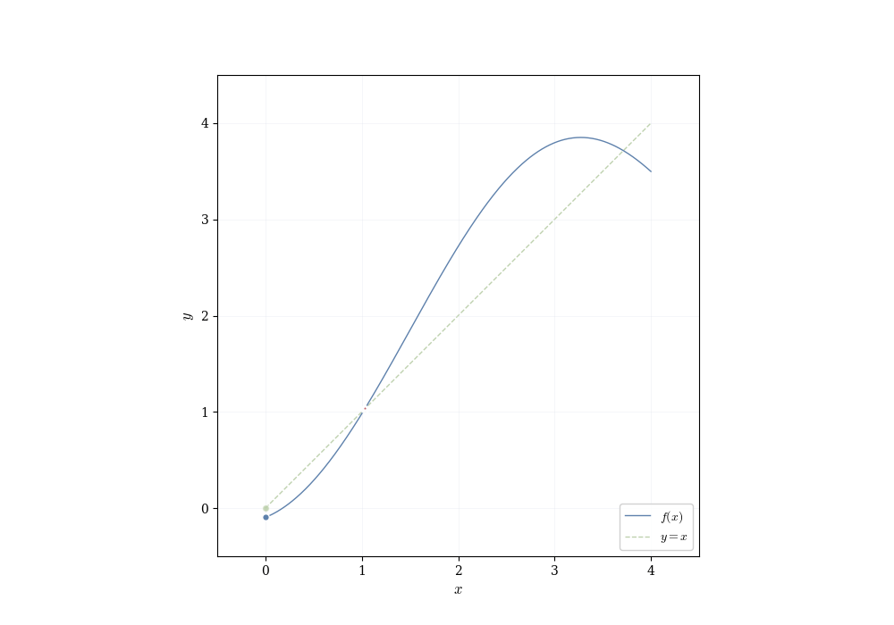
A related application concerns fixed points. Theorem 7.3 implies that if f : [a,b] \to [a,b] is continuous, then f has a fixed point, meaning some c \in [a,b] with f(c) = c.
Theorem 7.4 (Fixed Point Theorem (One Dimension)) Let f : [a,b] \to [a,b] be continuous. Then there exists c \in [a,b] such that f(c) = c.
Define g(x) = f(x) - x on [a,b]. Then g is continuous as the difference of continuous functions. Observe that g(a) = f(a) - a \geq 0 \quad \text{(since } f(a) \in [a,b] \text{)}, g(b) = f(b) - b \leq 0 \quad \text{(since } f(b) \in [a,b] \text{)}.
If g(a) = 0 or g(b) = 0, we have a fixed point at a or b. Otherwise, g(a) > 0 and g(b) < 0, so by Theorem 7.3, there exists c \in (a,b) with g(c) = 0, that is, f(c) = c. \square
7.6.3 Limitations and Extensions
Theorem 7.3 requires continuity on a closed bounded interval. Relaxing either condition can cause the conclusion to fail. The function f(x) = 1/x on (0,1) is continuous but takes no value between f(0^+) = +\infty and f(1) = 1; the interval is not closed. The function h(x) = \begin{cases} 0 & x < 1/2 \\ 1 & x \geq 1/2 \end{cases} on [0,1] fails to take the value 1/2 because it is not continuous.
Continuity on a closed interval, however, suffices even if the interval is unbounded or the function is not bounded. For instance, f(x) = \arctan x is continuous on \mathbb{R} and satisfies \lim_{x \to -\infty} f(x) = -\pi/2 and \lim_{x \to \infty} f(x) = \pi/2. For any y \in (-\pi/2, \pi/2), there exists c \in \mathbb{R} with f(c) = y. The essential ingredient is continuity, not boundedness of domain or range.
7.7 The Extreme Value Theorem
Continuous functions on closed bounded intervals cannot escape to infinity, nor can they oscillate wildly without bound. This observation, combined with the structure of the real numbers, ensures that such functions attain both a maximum and a minimum value.
Consider f(x) = x^2 on [0,2]. The function achieves its minimum value 0 at x=0 and its maximum value 4 at x=2. By contrast, g(x) = x^2 on the open interval (0,2) has no minimum: the values approach but never reach 0 as x \to 0^+. Similarly, h(x) = 1/x on (0,1] is continuous but has no maximum, as it grows without bound near x=0.
Theorem 7.5 guarantees that on a closed bounded interval, continuity forces the function to attain its bounds. There is no “escape route” to infinity, and no missing endpoint where an extremum might hide.
Theorem 7.5 (Extreme Value Theorem) Let f : [a,b] \to \mathbb{R} be continuous. Then there exist points c, d \in [a,b] such that f(c) \leq f(x) \leq f(d) \quad \text{for all } x \in [a,b].
That is, f attains both a maximum value f(d) and a minimum value f(c) on the interval.
The interval [a,b] is closed and bounded. We show that the image f([a,b]) inherits these properties, which forces the extreme values to be attained.
Boundedness: Suppose f([a,b]) were unbounded. Then for each n \in \mathbb{N}, there exists x_n \in [a,b] with |f(x_n)| > n. Because [a,b] is bounded, the points x_n cannot run off to infinity; they remain within [a,b]. By continuity, the function values cannot “jump” from finite points to infinity in one step, which is a contradiction. Hence f([a,b]) is bounded.
Closedness: Let y be a value that f gets arbitrarily close to on [a,b]. That is, for every 1/n > 0, there exists x_n \in [a,b] with |f(x_n) - y| < 1/n. Because [a,b] is closed, these points x_n stay inside the interval, and continuity guarantees that f actually takes the value y somewhere in [a,b]. Therefore f([a,b]) is closed.
Since f([a,b]) is a closed bounded subset of \mathbb{R}, it contains both its least and greatest elements. These correspond to the minimum and maximum values of f, attained at some points c, d \in [a,b]. \square
We have not been rigorous in the preceding argument. Implicitly, it relies on the Heine-Borel theorem. The preceding reasoning shows that the continuous image of a compact set is compact, hence closed and bounded. For [a,b], this ensures that f([a,b]) attains both its maximum and minimum values at some points c,d \in [a,b].
7.7.1 Necessity of the Hypotheses
All three conditions—continuity, closed interval, bounded interval—are necessary.
Without continuity: The function f(x) = \begin{cases} x & 0 \leq x < 1 \\ 0 & x = 1 \end{cases} on [0,1] is not continuous at x=1. The values approach but never reach 1, so there is no maximum. The supremum 1 is not attained.
Without closed interval: The function g(x) = x^2 on (0,1) is continuous but has neither a maximum (values approach 1 as x \to 1^-) nor a minimum (values approach 0 as x \to 0^+). The endpoints, where extrema would occur, are missing.
Without bounded interval: The function h(x) = x on [0,\infty) is continuous on a closed interval but unbounded. It has a minimum at x=0 but no maximum.
Each condition plays a role: continuity prevents jumps that would allow the function to skip over potential extrema, the closed interval ensures endpoints are included, and boundedness confines the function to a finite region where extrema must exist.
7.8 Applications to Optimization
Theorem 7.5 is the foundation of optimization. If a quantity depends continuously on a parameter that varies over a closed bounded interval, the theorem guarantees the existence of optimal values. We may not know how to find them analytically, but we know they exist. For techniques to find these extrema using derivatives, see ?sec-optimization.
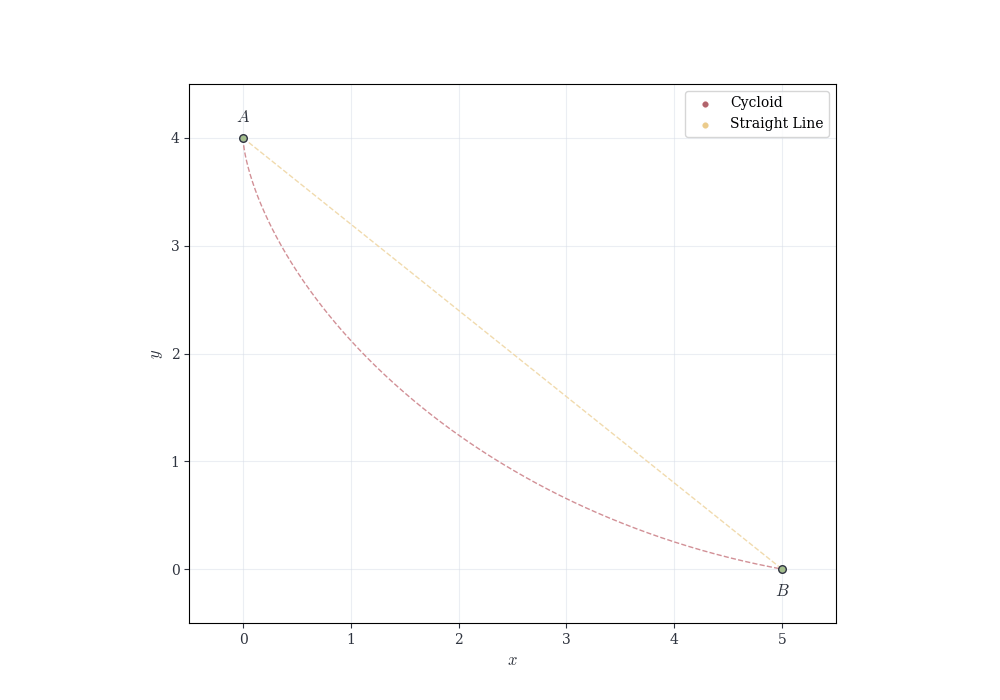
Example 7.4 (The Brachistochrone Problem) In 1696, Johann Bernoulli posed the problem: given two points A and B in a vertical plane, determine the curve along which a particle, moving under gravity alone, travels from A to B in the shortest time.
The travel time along a smooth curve \gamma is a continuous functional T(\gamma). While the Theorem 7.5 as stated applies to continuous real-valued functions on closed bounded intervals, the same principle—that continuous functions attain extrema on compact sets—extends to appropriate function spaces. With suitable compactness conditions on the admissible curves, one can guarantee that a minimizing curve exists. Johann Bernoulli showed it is a cycloid (the curve traced by a point on a rolling wheel).
Example 7.5 (Optimal Angle for Projectile Range) A projectile is launched with speed v_0 from the ground. Its horizontal range as a function of launch angle \theta \in [0, \pi/2] is R(\theta) = \frac{v_0^2 \sin(2\theta)}{g}.
The domain [0, \pi/2] is closed and bounded, and R is continuous on this interval. By Theorem 7.5, R attains a maximum.
Consider the function f(x) = \frac{x^2 - 4}{x - 2} for x \neq 2.
Explain why f is not defined at x = 2, but \lim_{x \to 2} f(x) exists. Compute this limit.
Define a new function g(x) by setting g(x) = f(x) for x \neq 2 and g(2) = L, where L is the limit you found in part (a). Prove using the \varepsilon-\delta definition (Definition 7.1) that g is continuous at x = 2.
Let (x_n) be any sequence with x_n \neq 2 for all n and x_n \to 2. Use Theorem 7.1 to explain why g(x_n) \to g(2).
Explain the difference between “removing a discontinuity” (as we did with g) versus “the function being continuous” (as with f). Why do we say f has a “removable discontinuity” at x = 2?
Consider the piecewise function h(x) = \begin{cases} x^2 - 1 & \text{if } x < 1 \\ ax + b & \text{if } x \geq 1 \end{cases} where a, b \in \mathbb{R} are constants to be determined.
For h to be continuous at x = 1, what equation must a and b satisfy? (Hint: Consider \lim_{x \to 1^-} h(x), \lim_{x \to 1^+} h(x), and h(1).)
Suppose we require additionally that the function passes through the point (2, 5). Find the unique values of a and b that make h continuous at x = 1 and satisfy h(2) = 5.
With your values from part (b), verify that h is continuous on all of \mathbb{R} by explaining why h is continuous at every point in (-\infty, 1), every point in (1, \infty), and at the transition point x = 1.
Use Theorem 7.3 to prove that h(x) = 2 has at least one solution in [0, 2]. (Check the values at the endpoints and apply the theorem.)
In this problem, you will prove a useful result about continuous functions that are bounded away from zero.
State the result. Complete the following theorem statement:
Theorem. Let f : [a, b] \to \mathbb{R} be continuous, and suppose f(x) \neq 0 for all x \in [a, b]. Then there exists \delta > 0 such that |f(x)| \geq \delta for all x \in [a, b].
In your own words, explain what this theorem says geometrically about the graph of f.
Prove existence of a minimum. Use Theorem 7.5 to explain why the function |f(x)| attains a minimum value on [a, b]. Call this minimum value m, and let c \in [a, b] be a point where |f(c)| = m.
Show the minimum is positive. Explain why m > 0. (Hint: What would happen if m = 0? Use the hypothesis that f(x) \neq 0 for all x.)
Complete the proof. Conclude that \delta = m satisfies the theorem. Explain why this means |f(x)| \geq m > 0 for all x \in [a, b].
Apply your result. Use your theorem to explain why the function g(x) = \frac{1}{x^2 + 1} is bounded on [0, 10]. Specifically, find a value of M > 0 such that |g(x)| \leq M for all x \in [0, 10].
Direct substitution gives f(2) = \frac{4 - 4}{2 - 2} = \frac{0}{0}, which is undefined. However, for x \neq 2, we can factor: f(x) = \frac{x^2 - 4}{x - 2} = \frac{(x-2)(x+2)}{x - 2} = x + 2.
Therefore, \lim_{x \to 2} f(x) = \lim_{x \to 2} (x + 2) = 4.
Proof. We have g(x) = x + 2 for x \neq 2 and g(2) = 4. In fact, g(x) = x + 2 for all x \in \mathbb{R}.
Let \varepsilon > 0. We must find \delta > 0 such that |x - 2| < \delta implies |g(x) - g(2)| < \varepsilon.
For any x \in \mathbb{R}, |g(x) - g(2)| = |(x + 2) - 4| = |x - 2|.
Choose \delta = \varepsilon. Then whenever |x - 2| < \delta, |g(x) - g(2)| = |x - 2| < \delta = \varepsilon.
Therefore g is continuous at x = 2. \square
By Theorem 7.1, since g is continuous at x = 2, for every sequence (x_n) with x_n \to 2, we have g(x_n) \to g(2).
More explicitly: the condition x_n \neq 2 ensures that g(x_n) = x_n + 2 for all n. As x_n \to 2, we have g(x_n) = x_n + 2 \to 2 + 2 = 4 = g(2).
The sequential characterization confirms that g is continuous at 2 by verifying the limit behavior along every possible sequence approaching 2.
The function f is not continuous at x = 2 because f(2) is not defined—continuity requires that the function be defined at the point in question.
However, the discontinuity is “removable” because the limit \lim_{x \to 2} f(x) exists. By defining g(2) = 4 (the value of the limit), we “fill in the hole” and create a continuous function g.
A removable discontinuity occurs when a function has a limit at a point but either (1) the function is undefined there, or (2) the function value doesn’t equal the limit. In either case, we can “remove” the discontinuity by redefining the function at that single point to equal the limit.
This is different from a jump discontinuity (like the Heaviside function at x = 0) or an essential discontinuity (like \sin(1/x) at x = 0), where no single value would make the function continuous.
For h to be continuous at x = 1, we need
\lim_{x \to 1^-} h(x) = \lim_{x \to 1^+} h(x) = h(1).
The left-hand limit
\lim_{x \to 1^-} h(x) = \lim_{x \to 1^-} (x^2 - 1) = 0.
The right-hand limit and function value \lim_{x \to 1^+} h(x) = \lim_{x \to 1^+} (ax + b) = a + b, \quad h(1) = a(1) + b = a + b.
Therefore, we need a + b = 0.
We have two conditions
Continuity at x = 1: a + b = 0
Pass through (2, 5): h(2) = 2a + b = 5
From the first equation, b = -a. Substituting into the second: 2a + (-a) = 5 \implies a = 5.
Therefore a = 5 and b = -5.
With a = 5 and b = -5, the function becomes h(x) = \begin{cases} x^2 - 1 & \text{if } x < 1 \\ 5x - 5 & \text{if } x \geq 1 \end{cases}
For any x_0 < 1, h(x) = x^2 - 1 in a neighborhood of x_0, which is continuous (polynomial).
For any x_0 > 1, h(x) = 5x - 5 in a neighborhood of x_0, which is continuous (linear).
At x = 1, we verified in part (a) that the left limit, right limit, and function value all equal 0, so h is continuous at x = 1.
By Theorem 7.2, polynomials and linear functions are continuous wherever they’re defined, and we’ve verified continuity at the transition point. Therefore h is continuous on all of \mathbb{R}.
We apply Theorem 7.3 with y = 2, a = 0, and b = 2.
First, compute the endpoint values: h(0) = 0^2 - 1 = -1, \quad h(2) = 5(2) - 5 = 5.
Since h is continuous on [0, 2] (by part (c)) and -1 < 2 < 5, Theorem 7.3 guarantees that there exists c \in (0, 2) such that h(c) = 2.
Therefore, the equation h(x) = 2 has at least one solution in [0, 2].
The theorem states that if f is continuous on a closed interval [a, b] and never equals zero, then f is bounded away from zero—there’s a positive lower bound \delta such that |f(x)| \geq \delta for all x.
Geometric interpretation: The graph of f never touches the x-axis, and in fact, it stays at least a distance \delta away from the x-axis. There’s no point where the function gets arbitrarily close to zero; it maintains a “safe distance” from zero throughout the entire interval.
Application of EVT. Consider the function g(x) = |f(x)| on [a, b]. Since f is continuous, g is continuous (composition of continuous functions—absolute value is continuous, see Theorem 7.2).
By Theorem 7.5, since g is continuous on the closed, bounded interval [a, b], g attains both a maximum and a minimum value. Let m denote the minimum value of g, and let c \in [a, b] be a point where this minimum occurs: m = g(c) = |f(c)| = \min_{x \in [a,b]} |f(x)|.
Minimum is positive. Suppose, for contradiction, that m = 0. Then |f(c)| = 0, which implies f(c) = 0.
But this contradicts the hypothesis that f(x) \neq 0 for all x \in [a, b]. Since c \in [a, b], we must have f(c) \neq 0, hence |f(c)| > 0.
Therefore m = |f(c)| > 0.
Completion of proof. Set \delta = m. Since m is the minimum value of |f(x)| on [a, b], we have |f(x)| \geq m = \delta \quad \text{for all } x \in [a, b].
From part (c), \delta = m > 0. This completes the proof: we’ve shown that there exists \delta > 0 such that |f(x)| \geq \delta for all x \in [a, b]. \square
This result is useful because it tells us that if a continuous function on a closed interval never equals zero, then we can safely divide by it—the reciprocal 1/f(x) is bounded on the interval.
The function g(x) = \frac{1}{x^2 + 1} is continuous on [0, 10] (it’s a composition of continuous functions—polynomial and reciprocal, with denominator x^2 + 1 \geq 1 > 0).
By Theorem 7.5, g attains a maximum on [0, 10]. Since x^2 + 1 is increasing on [0, 10], g(x) = 1/(x^2 + 1) is decreasing, so the maximum occurs at x = 0: g(x) \leq g(0) = \frac{1}{0 + 1} = 1 \quad \text{for all } x \in [0, 10].
Therefore M = 1 satisfies |g(x)| \leq M for all x \in [0, 10].
Additionally, since g(x) > 0 for all x \in [0, 10], the theorem from parts (a)–(d) gives a lower bound: g(x) \geq g(10) = \frac{1}{101} for all x \in [0, 10]. So g is bounded both above (by M = 1) and away from zero (by \delta = 1/101).