4 Limits of Real Functions
In the preceding chapters, we studied sequences—functions from the natural numbers to the real line. We asked: given a_n, does there exist a real number a such that a_n approaches a as n grows large? The \varepsilon-N machinery formalized this intuition, and we proved fundamental theorems governing convergent sequences.
Yet sequences capture only discrete processes. Consider again the motivating examples from Section 2.1
A biologist records bacterial population each day: P_1, P_2, P_3, \dots These measurements form a sequence; however, the underlying bacterial growth is continuous—between measurements at t = 5 and t = 6, the population evolves smoothly.
A physicist measures a particle’s position at integer times t = 0, 1, 2, \dots, producing a sequence s_0, s_1, s_2, \dots But the particle moves through all intermediate positions between these snapshots.
A patient’s blood pressure is monitored weekly. The measurements form a sequence, yet cardiovascular function is a continuous physiological process.
In each case, the discrete sequence is an approximation of an underlying continuous phenomenon. To model reality, we must study functions defined on continuous domains—intervals of real numbers rather than isolated integers.
This chapter extends the limit concept from sequences to functions f : \mathbb{R} \to \mathbb{R}. The guiding question shifts
Sequences: Does a_n approach a as n \to \infty?
Functions: Does f(x) approach L as x \to a?
The mathematical framework remains nearly identical. Where we previously required |a_n - a| < \varepsilon for all sufficiently large n, we now require |f(x) - L| < \varepsilon for all x sufficiently close to a. The discrete threshold N is replaced by a continuous tolerance \delta. This parallels the transition from discrete measurements to continuous observation.
4.1 Motivation: Instantaneous Velocity
To ground the notion of a limit, consider a concrete physical problem: determining the instantaneous velocity of a moving object.
Suppose a particle moves along a line, and its position at time t is given by s(t). The average velocity over the interval [t_0, t_0 + h] is
\bar{v} = \frac{s(t_0 + h) - s(t_0)}{h}.
This is the displacement divided by elapsed time—familiar from elementary physics.
But what is the particle’s velocity at the instant t = t_0? Setting h = 0 yields the meaningless expression \frac{0}{0}. Yet intuitively, we expect the particle to possess a well-defined velocity at each moment.
The resolution: examine what happens as h becomes arbitrarily small. If the average velocity v_{\text{avg}} approaches a definite value as h \to 0, we declare that value to be the instantaneous velocity at t_0. Formally,
v(t_0) = \lim_{h \to 0} \frac{s(t_0 + h) - s(t_0)}{h},
provided this limit exists.
This is not a sequence limit—h varies continuously through all real numbers near zero, not just integers. We require a new definition.
4.2 The Limit of a Function
We now formalize the notion of a function approaching a limit.
Definition 4.1 (Limit of a Function (Informal)) Let f be a function defined on an open interval containing a, except possibly at a itself. We say that
\lim_{x \to a} f(x) = L
if f(x) can be made arbitrarily close to L by taking x sufficiently close to a (but not equal to a).
This informal definition captures the intuition: as x approaches a, the values f(x) cluster around L. Crucially, the value f(a) itself is irrelevant—f need not even be defined at a.
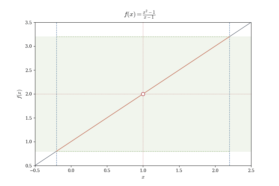
Example 4.1 (Limit Where Function is Undefined) Consider
f(x) = \frac{x^2 - 1}{x - 1}.
At x = 1, the denominator vanishes, so f(1) is undefined. Yet for x \neq 1,
f(x) = \frac{(x-1)(x+1)}{x-1} = x + 1.
As x approaches 1, f(x) approaches 2. We write \lim_{x \to 1} f(x) = 2, despite f(1) being undefined.
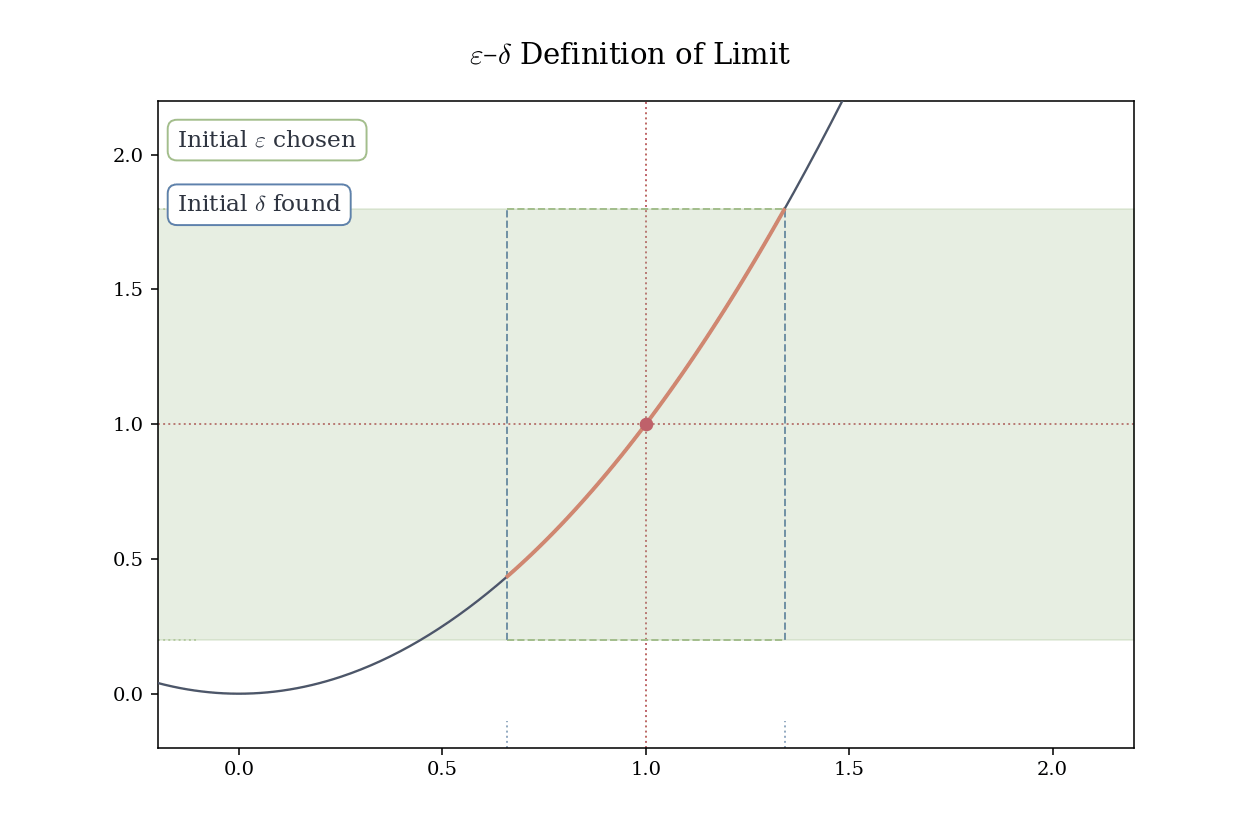
4.3 The \varepsilon-\delta Definition
The informal definition suffices for intuition, but in mathematics we demand precision. What does “arbitrarily close” and “sufficiently close” mean quantitatively?
Recall the \varepsilon-N definition of sequence convergence: for every tolerance \varepsilon > 0, there exists a threshold N such that all terms beyond N lie within \varepsilon of the limit.
For functions, we replace the integer threshold N with a distance threshold \delta > 0. The value f(x) must lie within \varepsilon of L whenever x lies within \delta of a (excluding a itself).
Definition 4.2 (Limit of a Function) Let f be defined on an open set U \subseteq \mathbb{R} (except possibly at a \in U), and let L \in \mathbb{R}. We say \lim_{x \to a} f(x) = L if for every \varepsilon > 0 there exists \delta > 0 such that 0 < |x-a| < \delta, \ x \in U \implies |f(x)-L| < \varepsilon.
Note: The statement |x - a| < \delta means x lies in the interval (a - \delta, a + \delta). While 0 < |x - a| excludes x = a itself. The function’s value at a is not relevant; only its behavior near a matters. Finally, |f(x) - L| < \varepsilon means f(x) lies in the interval (L - \varepsilon, L + \varepsilon).
The definition asserts: no matter how tight the tolerance \varepsilon, we can find a neighborhood around a (of radius \delta) such that all f(x) values within that neighborhood (excluding a) are within \varepsilon of L.
Example 4.2 (Limit of a Linear Function) Let f(x) = 2x + 3. We show that \lim_{x \to 1} f(x) = 5.
Proof. Let \varepsilon > 0. Set \delta = \varepsilon/2. Then for 0 < |x - 1| < \delta,
|f(x) - 5| = |2x + 3 - 5| = 2|x - 1| < 2 \cdot \frac{\varepsilon}{2} = \varepsilon.
Hence, \lim_{x \to 1} f(x) = 5. \square
TipScratch Work
We want 0 < |x - 1| < \delta \implies |f(x) - 5| < \varepsilon.
|f(x) - 5| = |2x + 3 - 5| = 2|x - 1|.
Require 2|x - 1| < \varepsilon, hence
|x - 1| < \frac{\varepsilon}{2}.
This motivates our choice
\delta = \frac{\varepsilon}{2}.
Interpretation
For a linear function, the “response” |f(x) - L| is proportional to the “perturbation” |x - a|. The proportionality constant (here, 2) determines how tightly \delta must be chosen relative to \varepsilon. That is, smaller tolerances \varepsilon require proportionally smaller neighborhoods \delta around a. (For numerical exploration, our limit calculator can evaluate limits step by step.)
It is useful to relate the \varepsilon–\delta definition of a limit to the behavior of a function along sequences. The idea of letting x approach p is naturally expressed by taking a sequence of points that converges to p, and many intuitive arguments in elementary calculus proceed in this way even if the language of sequences is not mentioned. The following theorem makes this connection precise. It shows that the limit of a function at a point is completely determined by the values of the function on all sequences converging to that point.
Theorem 4.1 (Sequential Criterion for Limits) Let E\subset\mathbb{R}, f:E\to\mathbb{R}, and let p be a limit point of E. The following two statements are equivalent
\lim_{x\to p} f(x)=q.
For every sequence (p_n) in E with p_n\neq p for all n and p_n\to p, we have f(p_n)\to q.
TipProof.
(\Rightarrow) Assume first that \lim_{x\to p} f(x)=q. Fix \varepsilon>0. By the definition of the limit, there is a \delta>0 such that |f(x)-q|<\varepsilon whenever x\in E and 0<|x-p|<\delta. If (p_n) is any sequence in E with p_n\neq p and p_n\to p, then there is N such that |p_n-p|<\delta for all n>N. For such n we have |f(p_n)-q|<\varepsilon, so f(p_n)\to q.
(\Leftarrow) For the converse, assume the limit does not exist. Then there is some \varepsilon>0 such that for every \delta>0 we can find x\in E with 0<|x-p|<\delta and |f(x)-q|\ge\varepsilon. Define a sequence (p_n) by choosing each p_n\in E so that 0<|p_n-p|<1/n and |f(p_n)-q|\ge\varepsilon. Then p_n\to p, but |f(p_n)-q|\ge\varepsilon for all n, so f(p_n) does not converge to q, contradicting (2). Thus the limit must exist and equal q. \square
It is natural to ask whether a function can approach two distinct values at the same point. By analogy with sequences, whose limits are unique (see Theorem 3.1), one expects the same for functions. Indeed, if \lim_{x \to a} f(x) exists, it is unique. No function can converge to two different values at the same point; any assumption to the contrary immediately contradicts the uniqueness of sequence limits. This fundamental fact underlies all further considerations of limits.
Theorem 4.2 (Uniqueness of Limits of Functions) Let f: U \to \mathbb{R} with U \subset \mathbb{R}, and let a be a limit point of U. If \lim_{x \to a} f(x) = L_1 \quad \text{and} \quad \lim_{x \to a} f(x) = L_2, then L_1 = L_2.
TipProof.
Suppose, for contradiction, that L_1 \neq L_2, and set \varepsilon = |L_1 - L_2|/2 > 0. By definition, there exist \delta_1, \delta_2 > 0 such that
0 < |x - a| < \delta_1 \implies |f(x) - L_1| < \varepsilon, \quad 0 < |x - a| < \delta_2 \implies |f(x) - L_2| < \varepsilon.
Let \delta = \min(\delta_1, \delta_2). For any x with 0 < |x - a| < \delta, both inequalities hold, so by the triangle inequality,
|L_1 - L_2| \le |f(x) - L_1| + |f(x) - L_2| < 2 \varepsilon = |L_1 - L_2|,
a contradiction. Hence L_1 = L_2. \square
4.4 One-Sided Limits
Sometimes a function behaves differently as x approaches a from the left versus from the right. We introduce one-sided limits to capture this distinction.
Definition 4.3 (One-Sided Limits) We say
\lim_{x \to a^-} f(x) = L
if for every \varepsilon > 0 there exists \delta > 0 such that
a - \delta < x < a \implies |f(x) - L| < \varepsilon.
Similarly,
\lim_{x \to a^+} f(x) = L
if for every \varepsilon > 0 there exists \delta > 0 such that
a < x < a + \delta \implies |f(x) - L| < \varepsilon.
Theorem 4.3 (Two-Sided Limit via One-Sided Limits) If both one-sided limits of f at c exist and are equal, then the two-sided limit exists and equals this common value.
TipProof.
Let L be the common value. Given \varepsilon > 0, choose \delta^+ > 0 and \delta^- > 0 such that
|f(x) - L| < \varepsilon \quad \text{whenever } 0 < x - c < \delta^+ \text{ or } 0 < c - x < \delta^-.
Set
\delta = \min(\delta^-, \delta^+).
Then for all x with 0 < |x - c| < \delta, x lies on one side of c, so |f(x) - L| < \varepsilon. Hence f(x) \to L as x \to c. \square
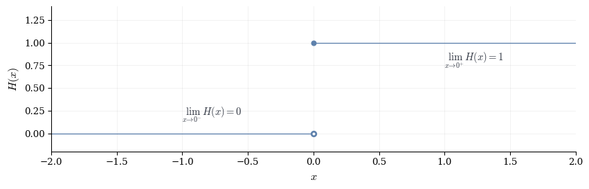
Example 4.3 (The Heaviside Step Function) Define
H(x) = \begin{cases} 0 & \text{if } x < 0, \\ 1 & \text{if } x \ge 0. \end{cases}
At x = 0
- \lim_{x \to 0^-} H(x) = 0 (approaching from the left, H(x) = 0)
- \lim_{x \to 0^+} H(x) = 1 (approaching from the right, H(x) = 1)
Since the one-sided limits differ, \lim_{x \to 0} H(x) does not exist.
WarningProblem Set
Let f(x) = 3x + 2 and consider \lim_{x \to 1} f(x).
Use the \varepsilon-\delta definition to prove that \lim_{x \to 1} f(x) = 5.
For \varepsilon = 0.15, find explicitly a value of \delta > 0 that works in the \varepsilon-\delta definition.
Explain in words why the relationship \delta = \varepsilon/3 works for this function.
If we change the function to g(x) = 5x + 2, what would be the corresponding relationship between \delta and \varepsilon for proving \lim_{x \to 1} g(x) = 7? Explain your reasoning.
Consider the function f(x) = \frac{x^2 + 3x - 4}{x - 1}.
Show that f(x) can be simplified to x + 4 for all x \neq 1.
Use this simplification to determine \lim_{x \to 1} f(x).
Explain why the fact that f(1) is undefined does not prevent the limit from existing.
Let (x_n) be any sequence with x_n \neq 1 for all n and x_n \to 1. Use Theorem 4.1 to explain what happens to f(x_n) as n \to \infty.
Define the function h(x) = \begin{cases} x^2 & \text{if } x < 2 \\ 6 & \text{if } x = 2 \\ 2x & \text{if } x > 2 \end{cases}
Compute \lim_{x \to 2^-} h(x) and \lim_{x \to 2^+} h(x).
Does \lim_{x \to 2} h(x) exist? Justify your answer using Theorem 4.3.
How is the value h(2) = 6 related (or not related) to your answer in part (b)?
Modify the definition of h(x) for x > 2 so that the two-sided limit \lim_{x \to 2} h(x) exists. What must the common value of the one-sided limits be?
WarningSolutions
Proof. Let \varepsilon > 0. We seek \delta > 0 such that 0 < |x - 1| < \delta \implies |f(x) - 5| < \varepsilon.
Observe that |f(x) - 5| = |3x + 2 - 5| = |3x - 3| = 3|x - 1|.
To ensure 3|x - 1| < \varepsilon, we require |x - 1| < \varepsilon/3.
Therefore, choose \delta = \varepsilon/3. Then for 0 < |x - 1| < \delta, |f(x) - 5| = 3|x - 1| < 3 \cdot \frac{\varepsilon}{3} = \varepsilon.
Hence \lim_{x \to 1} f(x) = 5. \square
For \varepsilon = 0.15, we use \delta = \varepsilon/3 = 0.15/3 = 0.05.
Thus \delta = 0.05 works: whenever 0 < |x - 1| < 0.05, we have |f(x) - 5| < 0.15.
The function f(x) = 3x + 2 has slope 3. This means that when x changes by an amount \Delta x, the function value changes by 3\Delta x. To keep the change in f(x) below \varepsilon, we need 3\Delta x < \varepsilon, which gives \Delta x < \varepsilon/3. This is precisely why \delta = \varepsilon/3 works.
The function g(x) = 5x + 2 has slope 5. Following the same reasoning as in part (c), we would have |g(x) - 7| = |5x + 2 - 7| = |5x - 5| = 5|x - 1|.
To ensure 5|x - 1| < \varepsilon, we need |x - 1| < \varepsilon/5.
Therefore the relationship would be \delta = \varepsilon/5. The larger slope (5 versus 3) means we need a smaller neighborhood around a = 1 to control the function’s behavior within the same tolerance \varepsilon.
Factor the numerator: x^2 + 3x - 4 = (x - 1)(x + 4).
Therefore, for x \neq 1, f(x) = \frac{(x-1)(x+4)}{x-1} = x + 4.
Using the simplification from part (a), for x \neq 1 we have f(x) = x + 4. As x \to 1, \lim_{x \to 1} f(x) = \lim_{x \to 1} (x + 4) = 1 + 4 = 5.
The \varepsilon-\delta definition of the limit (Definition 4.2) requires 0 < |x - a| < \delta, which explicitly excludes x = a. The limit describes the behavior of f(x) as x approaches a, not the value at a. Since we never evaluate f at x = 1 in taking the limit, whether f(1) is defined, undefined, or defined with some other value is irrelevant to the existence of the limit.
By Theorem 4.1, if \lim_{x \to 1} f(x) = 5 and (x_n) is any sequence with x_n \neq 1 and x_n \to 1, then f(x_n) \to 5.
More explicitly: since x_n \neq 1 for all n, we can use the simplified form f(x_n) = x_n + 4. As x_n \to 1, we have f(x_n) = x_n + 4 \to 1 + 4 = 5.
This confirms that the sequence of function values converges to the limit, even though the function is never actually evaluated at x = 1.
For the left-hand limit, as x \to 2^-, we use the formula h(x) = x^2: \lim_{x \to 2^-} h(x) = \lim_{x \to 2^-} x^2 = 4.
For the right-hand limit, as x \to 2^+, we use the formula h(x) = 2x: \lim_{x \to 2^+} h(x) = \lim_{x \to 2^+} 2x = 4.
Yes, \lim_{x \to 2} h(x) exists and equals 4.
By Theorem 4.3, if both one-sided limits exist and are equal, then the two-sided limit exists and equals their common value. Since \lim_{x \to 2^-} h(x) = 4 = \lim_{x \to 2^+} h(x), we conclude that \lim_{x \to 2} h(x) = 4.
The value h(2) = 6 is not related to the limit. The limit depends only on the behavior of h(x) as x approaches 2, not on the value at x = 2 itself. The function happens to be defined at x = 2 with value 6, but this plays no role in determining \lim_{x \to 2} h(x) = 4.
In fact, h(2) \neq \lim_{x \to 2} h(x), which means h is not continuous at x = 2 (as we will study in the next chapter).
For the two-sided limit to exist, the one-sided limits must be equal. We found in part (a) that \lim_{x \to 2^-} h(x) = 4, so we need \lim_{x \to 2^+} h(x) = 4 as well.
Currently, for x > 2, we have h(x) = 2x, which gives \lim_{x \to 2^+} h(x) = 4. This already works!
More generally, any formula g(x) for x > 2 with \lim_{x \to 2^+} g(x) = 4 would work. For example:
- h(x) = 4 for x > 2 (constant)
- h(x) = x^2 for x > 2 (matching the left piece)
- h(x) = 4 + (x-2)^2 for x > 2 (approaches 4 from above)
In all cases, the common value of the one-sided limits must be 4 to ensure the two-sided limit exists.