4 Linear Maps

A vector space is determined by which linear combinations it permits. A linear map is a function that preserves this structure—it sends linear combinations to linear combinations. The theory of linear maps governs how vector spaces relate to one another and provides the framework for solving systems of equations, studying transformations, and analyzing operators.

We work over \mathbb{R} unless stated otherwise. Throughout this chapter, \mathcal{V} and \mathcal{W} denote vector spaces.

4.1 Definition and Examples

In differential calculus, the differential df_a was a linear approximation to a function near a point. The derivative operator D : C^1([a,b]) \to C([a,b]) sending f \mapsto f' preserves addition and scaling: (f+g)' = f' + g' and (cf)' = cf'. Integration behaves similarly. These are instances of linear maps.

Definition 4.1 (Linear map) A function T : \mathcal{V} \to \mathcal{W} is a linear map if for all u,v \in \mathcal{V} and all c \in \mathbb{R}, T(u+v) = T(u) + T(v), \quad T(cv) = cT(v).

Equivalently, T is linear if T\left(\sum_{i=1}^{n} a_i v_i\right) = \sum_{i=1}^{n} a_i T(v_i) for all finite linear combinations.

The set of all linear maps from \mathcal{V} to \mathcal{W} is denoted \mathcal{L}(\mathcal{V}, \mathcal{W}).

Examples.

Identity map. I : \mathcal{V} \to \mathcal{V} defined by I(v) = v is linear.
Zero map. 0 : \mathcal{V} \to \mathcal{W} defined by 0(v) = 0 is linear.
Scalar multiplication. For fixed c \in \mathbb{R}, the map T : \mathcal{V} \to \mathcal{V} defined by T(v) = cv is linear.
Projection. In \mathbb{R}^2, the map T : \mathbb{R}^2 \to \mathbb{R}^2 defined by T\begin{pmatrix} x \\ y \end{pmatrix} = \begin{pmatrix} x \\ 0 \end{pmatrix} is linear. It projects onto the x-axis.
Differentiation. The map D : \mathcal{P}_n \to \mathcal{P}_{n-1} defined by D(p) = p' is linear.
Integration. The map I : C([a,b]) \to \mathbb{R} defined by I(f) = \int_a^b f(x) \, dx is a linear functional.

Theorem 4.1 If T : \mathcal{V} \to \mathcal{W} is linear, then T(0) = 0.

Proof. We have T(0) = T(0 \cdot v) = 0 \cdot T(v) = 0 for any v \in \mathcal{V}. \square

Theorem 4.2 \mathcal{L}(\mathcal{V}, \mathcal{W}) is a vector space under pointwise addition and scalar multiplication: (S+T)(v) = S(v) + T(v), \quad (cT)(v) = c \cdot T(v).

Proof. Verification of the vector space axioms reduces to properties of \mathcal{W}. For instance, \begin{align*} (S+T)(u+v) &= S(u+v) + T(u+v)\\ &= S(u) + S(v) + T(u) + T(v) \\ & = (S+T)(u) + (S+T)(v). \end{align*} The zero vector in \mathcal{L}(\mathcal{V}, \mathcal{W}) is the zero map. \square

Theorem 4.3 A linear map T : \mathcal{V} \to \mathcal{W} is uniquely determined by its values on a basis of \mathcal{V}.

Proof. Let \{e_i\}_{i=1}^n be a basis of \mathcal{V}. Then, any v \in \mathcal{V} can be written uniquely as v = \sum_{i=1}^{n} a_i e_i. Hence T(v) = T\left(\sum_{i=1}^{n} a_i e_i\right) = \sum_{i=1}^{n} a_i T(e_i). Thus T(v) is completely determined by the values T(e_1),\dots,T(e_n). Conversely, given any choice of vectors w_1,\dots,w_n \in \mathcal{W}, defining T(e_i) = w_i extends uniquely to a linear map on all of \mathcal{V} by the formula above. \square

4.2 Kernel and Image

A linear map T : \mathcal{V} \to \mathcal{W} produces two canonical subspaces: the set of vectors sent to zero, and the set of vectors in \mathcal{W} that arise as images.

Definition 4.2 (Kernel and image) Let T : \mathcal{V} \to \mathcal{W} be linear. The kernel of T is \ker(T) = \{ v \in \mathcal{V} : T(v) = 0 \}. The image of T is \operatorname{im}(T) = \{ T(v) : v \in \mathcal{V} \}.

Theorem 4.4 \ker(T) is a subspace of \mathcal{V} and \operatorname{im}(T) is a subspace of \mathcal{W}.

Proof. Since T(0) = 0, we have 0 \in \ker(T). If u,v \in \ker(T), then T(u+v) = T(u) + T(v) = 0 + 0 = 0, so u+v \in \ker(T). If v \in \ker(T) and c \in \mathbb{R}, then T(cv) = cT(v) = c \cdot 0 = 0, so cv \in \ker(T).

For the image, 0 = T(0) \in \operatorname{im}(T). If w_1, w_2 \in \operatorname{im}(T), write w_i = T(v_i). Then w_1 + w_2 = T(v_1) + T(v_2) = T(v_1 + v_2) \in \operatorname{im}(T). Scalar multiples behave similarly. \square

Examples.

For the projection T : \mathbb{R}^2 \to \mathbb{R}^2 defined by T\begin{pmatrix} x \\ y \end{pmatrix} = \begin{pmatrix} x \\ 0 \end{pmatrix}, we have \ker(T) = \left\{ \begin{pmatrix} 0 \\ y \end{pmatrix} : y \in \mathbb{R} \right\}, \quad \operatorname{im}(T) = \left\{ \begin{pmatrix} x \\ 0 \end{pmatrix} : x \in \mathbb{R} \right\}. Both are lines through the origin.
For differentiation D : \mathcal{P}_n \to \mathcal{P}_{n-1}, we have \ker(D) = \{c : c \in \mathbb{R}\} (constant polynomials) and \operatorname{im}(D) = \mathcal{P}_{n-1}.
For the zero map, \ker(0) = \mathcal{V} and \operatorname{im}(0) = \{0\}.

4.3 Rank and Nullity

The dimensions of kernel and image measure how much information T loses and produces.

Definition 4.3 (Rank and nullity) Let T : \mathcal{V} \to \mathcal{W} be linear with \mathcal{V} finite-dimensional. The nullity of T is \dim \ker(T). The rank of T is \dim \operatorname{im}(T).

Theorem 4.5 (Rank–nullity theorem) If T : \mathcal{V} \to \mathcal{W} is linear and \mathcal{V} is finite-dimensional, then \dim \mathcal{V} = \dim \ker(T) + \dim \operatorname{im}(T).

Proof. Let \{u_1,\dots,u_k\} be a basis of \ker(T). Extend it to a basis \{u_1,\dots,u_k, v_1,\dots,v_r\} of \mathcal{V}, so \dim \mathcal{V} = k + r.

We claim \{T(v_1),\dots,T(v_r)\} is a basis of \operatorname{im}(T).

Spanning. Let w \in \operatorname{im}(T). Then w = T(v) for some v = \sum_{i=1}^{k} a_i u_i + \sum_{j=1}^{r} b_j v_j. Applying T, w = T(v) = \sum_{i=1}^{k} a_i T(u_i) + \sum_{j=1}^{r} b_j T(v_j) = \sum_{j=1}^{r} b_j T(v_j) since T(u_i) = 0.

Independence. Suppose \sum_{j=1}^{r} c_j T(v_j) = 0. Then T\left(\sum_{j=1}^{r} c_j v_j\right) = 0, so \sum_{j=1}^{r} c_j v_j \in \ker(T). Thus \sum_{j=1}^{r} c_j v_j = \sum_{i=1}^{k} d_i u_i for some d_i. Rearranging, \sum_{i=1}^{k} (-d_i) u_i + \sum_{j=1}^{r} c_j v_j = 0. Since \{u_1,\dots,u_k, v_1,\dots,v_r\} is independent, c_j = 0 for all j.

Therefore \dim \operatorname{im}(T) = r = \dim \mathcal{V} - k = \dim \mathcal{V} - \dim \ker(T). \square

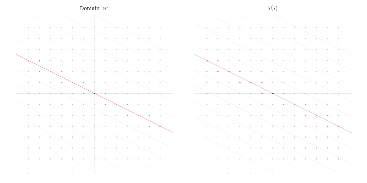
4.4 Injectivity and Surjectivity

The kernel and image control when T is injective or surjective.

Theorem 4.6 A linear map T : \mathcal{V} \to \mathcal{W} is injective if and only if \ker(T) = \{0\}.

Proof. Suppose T is injective. If v \in \ker(T), then T(v) = 0 = T(0), so v = 0 by injectivity.

Conversely, suppose \ker(T) = \{0\}. If T(u) = T(v), then T(u-v) = T(u) - T(v) = 0, so u - v \in \ker(T) = \{0\}. Thus u = v. \square

Theorem 4.7 A linear map T : \mathcal{V} \to \mathcal{W} is surjective if and only if \operatorname{im}(T) = \mathcal{W}.

Proof. Immediate from the definition. \square

Definition 4.4 (Isomorphism) A linear map T : \mathcal{V} \to \mathcal{W} is an isomorphism if it is bijective (injective and surjective). We say \mathcal{V} and \mathcal{W} are isomorphic, written \mathcal{V} \cong \mathcal{W}, if there exists an isomorphism between them.

An isomorphism is in some sense a “perfect” relabeling. Every vector in \mathcal{V} corresponds to exactly one vector in \mathcal{W}, and the correspondence preserves all linear structure. Isomorphic spaces are algebraically indistinguishable—they have the same dimension, the same behavior under linear operations, the same subspace structure. When \mathcal{V} \cong \mathcal{W}, any theorem true for \mathcal{V} holds for \mathcal{W} after relabeling.

The suffix “-morphism” recurs throughout mathematics. Diffeomorphisms preserve smooth structure, homeomorphisms preserve topological structure, group homomorphisms preserve group operations. In each case, a morphism is a map that respects the relevant structure, and an isomorphism is a bijective morphism establishing structural equivalence. Linear isomorphisms preserve vector space structure.

Theorem 4.8 If \mathcal{V} and \mathcal{W} are finite-dimensional, then \mathcal{V} \cong \mathcal{W} if and only if \dim \mathcal{V} = \dim \mathcal{W}.

Proof. Suppose T : \mathcal{V} \to \mathcal{W} is an isomorphism. By Theorem 4.6, \ker(T) = \{0\}, so \dim \ker(T) = 0. By Theorem 4.5, \dim \mathcal{V} = \dim \operatorname{im}(T). Since T is surjective, \operatorname{im}(T) = \mathcal{W}, giving \dim \mathcal{V} = \dim \mathcal{W}.

Conversely, suppose \dim \mathcal{V} = \dim \mathcal{W} = n. Let \{v_1,\dots,v_n\} be a basis of \mathcal{V} and \{w_1,\dots,w_n\} a basis of \mathcal{W}. Define T : \mathcal{V} \to \mathcal{W} by T\left(\sum_{i=1}^{n} a_i v_i\right) = \sum_{i=1}^{n} a_i w_i. This is linear. If T(v) = 0, then \sum a_i w_i = 0, so a_i = 0 for all i, giving v = 0. Thus \ker(T) = \{0\} and T is injective. By Theorem 4.5, \dim \operatorname{im}(T) = \dim \mathcal{V} - \dim \ker(T) = n, so \operatorname{im}(T) = \mathcal{W} and T is surjective. \square

Consequence. All n-dimensional vector spaces over \mathbb{R} are isomorphic to \mathbb{R}^n. Isomorphism is an equivalence relation partitioning vector spaces by dimension.

4.5 Composition

Linear maps compose naturally, and composition respects the linear structure.

Theorem 4.9 If T : \mathcal{V} \to \mathcal{W} and S : \mathcal{W} \to \mathcal{U} are linear, then S \circ T : \mathcal{V} \to \mathcal{U} is linear.

Proof. For u,v \in \mathcal{V} and c \in \mathbb{R}, \begin{align*} (S \circ T)(u+v) &= S(T(u+v)) \\ &= S(T(u) + T(v)) \\ &= S(T(u)) + S(T(v))\\ &= (S \circ T)(u) + (S \circ T)(v). \end{align*} Scalar multiplication follows similarly. \square

Theorem 4.10 A linear map T : \mathcal{V} \to \mathcal{W} is an isomorphism if and only if there exists a linear map S : \mathcal{W} \to \mathcal{V} such that S \circ T = I_{\mathcal{V}} and T \circ S = I_{\mathcal{W}}.

Proof. If such S exists, T is bijective: injectivity follows from T(v) = 0 \Rightarrow v = S(T(v)) = 0, and surjectivity from w = T(S(w)).

Conversely, if T is an isomorphism, the set-theoretic inverse T^{-1} : \mathcal{W} \to \mathcal{V} is well-defined. We verify it is linear. For w_1, w_2 \in \mathcal{W}, write w_i = T(v_i). Then T(v_1 + v_2) = T(v_1) + T(v_2) = w_1 + w_2, so T^{-1}(w_1 + w_2) = v_1 + v_2 = T^{-1}(w_1) + T^{-1}(w_2). Scalar multiplication follows similarly. \square

4.6 Direct Sums and Decompositions

The rank–nullity theorem implies \mathcal{V} = \ker(T) \oplus \mathcal{U} for some subspace \mathcal{U}. This decomposition simplifies many arguments.

Theorem 4.11 Let T : \mathcal{V} \to \mathcal{W} be linear with \mathcal{V} finite-dimensional. There exists a subspace \mathcal{U} \subseteq \mathcal{V} such that \mathcal{V} = \ker(T) \oplus \mathcal{U}. Moreover, T|_{\mathcal{U}} : \mathcal{U} \to \operatorname{im}(T) is an isomorphism.

Proof. In the proof of Theorem 4.5, we extended a basis \{u_1,\dots,u_k\} of \ker(T) to a basis of \mathcal{V} by adding \{v_1,\dots,v_r\}. Let \mathcal{U} = \operatorname{span}(v_1,\dots,v_r).

By construction, \mathcal{V} = \operatorname{span}(u_1,\dots,u_k, v_1,\dots,v_r) and \ker(T) \cap \mathcal{U} = \{0\} (independence of the extended basis). Thus \mathcal{V} = \ker(T) \oplus \mathcal{U}.

The map T|_{\mathcal{U}} : \mathcal{U} \to \operatorname{im}(T) is injective: if T(v) = 0 with v \in \mathcal{U}, then v \in \ker(T) \cap \mathcal{U} = \{0\}. It is surjective: we showed \{T(v_1),\dots,T(v_r)\} spans \operatorname{im}(T). \square

This decomposition appears throughout linear algebra. When analyzing T, we separate the kernel (where T annihilates) from a complement (where T is bijective onto its image).

4.7 Linear Functionals and the Dual Space

A linear map \varphi : \mathcal{V} \to \mathbb{R} assigns a scalar to each vector. Such maps are called linear functionals. In differential calculus, the differential df_a was a linear functional measuring approximate change. Integration \int_a^b f(x) \, dx is a linear functional on C([a,b]).

Definition 4.5 (Dual space) The dual space of \mathcal{V}, denoted \mathcal{V}^*, is the vector space \mathcal{L}(\mathcal{V}, \mathbb{R}) of all linear functionals on \mathcal{V}.

Theorem 4.12 If \mathcal{V} is finite-dimensional, then \dim \mathcal{V}^* = \dim \mathcal{V}.

Proof. Let \{v_1,\dots,v_n\} be a basis of \mathcal{V}. Define \varphi_i \in \mathcal{V}^* by \varphi_i\left(\sum_{j=1}^{n} a_j v_j\right) = a_i. Each \varphi_i is linear. We claim \{\varphi_1,\dots,\varphi_n\} is a basis of \mathcal{V}^*.

Independence: Suppose \sum_{i=1}^{n} c_i \varphi_i = 0. Evaluating on v_j, 0 = \left(\sum_{i=1}^{n} c_i \varphi_i\right)(v_j) = c_j, so all c_i = 0.

Spanning: Let \psi \in \mathcal{V}^*. Define c_i = \psi(v_i). Then for v = \sum_{j=1}^{n} a_j v_j, \psi(v) = \sum_{j=1}^{n} a_j \psi(v_j) = \sum_{j=1}^{n} a_j c_j = \sum_{i=1}^{n} c_i \varphi_i(v), so \psi = \sum_{i=1}^{n} c_i \varphi_i. \square

The functionals \{\varphi_1,\dots,\varphi_n\} are called the dual basis to \{v_1,\dots,v_n\}. They satisfy \varphi_i(v_j) = \delta_{ij}, where \delta_{ij} is the Kronecker delta: \delta_{ij} = \begin{cases} 1 & \text{if } i = j \\ 0 & \text{if } i \neq j \end{cases}. This property characterizes dual bases: each \varphi_i extracts the i-th coordinate with respect to the basis \{v_1,\dots,v_n\}.

4.8 The Transpose

A linear map T : \mathcal{V} \to \mathcal{W} induces a map on dual spaces going in the opposite direction.

Definition 4.6 (Transpose) Let T : \mathcal{V} \to \mathcal{W} be linear. The transpose (or dual) of T is the map T^* : \mathcal{W}^* \to \mathcal{V}^* defined by (T^* \varphi)(v) = \varphi(T(v)) for \varphi \in \mathcal{W}^* and v \in \mathcal{V}.

Theorem 4.13 T^* is linear.

Proof. For \varphi, \psi \in \mathcal{W}^* and c \in \mathbb{R}, (T^*(\varphi + \psi))(v) = (\varphi + \psi)(T(v)) = \varphi(T(v)) + \psi(T(v)) = (T^*\varphi)(v) + (T^*\psi)(v), so T^*(\varphi + \psi) = T^*\varphi + T^*\psi. Scalar multiplication follows similarly. \square

Theorem 4.14 If \mathcal{V} and \mathcal{W} are finite-dimensional, then \dim \operatorname{im}(T^*) = \dim \operatorname{im}(T).

Proof. A functional \varphi \in \mathcal{W}^* lies in \ker(T^*) if and only if (T^*\varphi)(v) = 0 for all v \in \mathcal{V}, equivalently \varphi(T(v)) = 0 for all v \in \mathcal{V}, equivalently \varphi vanishes on \operatorname{im}(T).

Let \{w_1,\dots,w_r\} be a basis of \operatorname{im}(T) and extend it to a basis \{w_1,\dots,w_r, w_{r+1},\dots,w_m\} of \mathcal{W}. Let \{\psi_1,\dots,\psi_m\} be the dual basis. Then \varphi vanishes on \operatorname{im}(T) if and only if \varphi(w_i) = 0 for i \le r. Writing \varphi = \sum_{j=1}^{m} c_j \psi_j and evaluating on w_i gives c_i = 0 for i \le r. Thus \ker(T^*) = \operatorname{span}(\psi_{r+1},\dots,\psi_m), so \dim \ker(T^*) = m - r.

By Theorem 4.5 applied to T^*, \dim \operatorname{im}(T^*) = \dim \mathcal{W}^* - \dim \ker(T^*) = m - (m - r) = r = \dim \operatorname{im}(T). \square

The transpose reverses arrows: T : \mathcal{V} \to \mathcal{W} induces T^* : \mathcal{W}^* \to \mathcal{V}^*. Composition reverses: (S \circ T)^* = T^* \circ S^*.

This reversal is called contravariance. Vectors transform covariantly: if T : \mathcal{V} \to \mathcal{W} and v \in \mathcal{V}, we get T(v) \in \mathcal{W}, following the arrow. Covectors (functionals) transform contravariantly: if \varphi \in \mathcal{W}^*, we get T^*\varphi \in \mathcal{V}^*, reversing the arrow.

Physically, vectors represent displacements or velocities—they transform with changes of coordinates. Covectors represent gradients or forces—they transform inversely. If you stretch coordinates by a factor of 2, displacements double but gradients halve. This distinction appears throughout differential geometry and physics: tangent vectors are contravariant, cotangent vectors (differentials) are covariant. In coordinates, contravariant components use upper indices v^i, covariant components use lower indices \varphi_i.

4.9 Closing Remarks

Linear maps between finite-dimensional spaces are controlled by their kernels and images. The rank–nullity theorem quantifies this relationship. Injectivity is equivalent to trivial kernel; surjectivity to full image. Isomorphisms exist precisely when dimensions match.

The dual space \mathcal{V}^* collects all linear functionals on \mathcal{V}, and the transpose T^* shows how functionals transform contravariantly to vectors.

In the next chapter we introduce matrices as coordinate representations of linear maps. The abstract theory developed here translates into explicit computations once bases are chosen.