14 Chapter: Discrete Dynamical Systems and Markov Chains
This chapter studies what happens when you apply a matrix repeatedly: x_0, Ax_0, A^2x_0, \ldots The question—does this sequence converge, diverge, or oscillate?—turns out to depend entirely on the eigenvalues of A. We develop this theory carefully, then apply it to Markov chains, population models, and discrete approximations of continuous systems.
Core material (Sections 1–4) is central to the course and should be read in full. Sections marked ★ introduce advanced applications—mixing times, quantum evolution, financial models—that illustrate the reach of spectral theory. These may be treated as enrichment or assigned selectively; no subsequent core material depends on them.
14.1 Sequences of Vectors and Linear Recurrences
A sequence of vectors in \mathbb{F}^d is a function \mathbb{N} \to \mathbb{F}^d, written (x_n)_{n=0}^\infty or simply (x_n) when the index set is understood. We write x_n = (x_n^{(1)}, \ldots, x_n^{(d)})^T \in \mathbb{F}^d to emphasize the d components of the n-th term.
Definition 14.1 (Convergence of vector sequences) A sequence (x_n) in \mathbb{F}^d converges to x \in \mathbb{F}^d if for every \varepsilon > 0 there exists N \in \mathbb{N} such that n \ge N \implies \|x_n - x\| < \varepsilon. We write \lim_{n \to \infty} x_n = x or x_n \to x.
The norm \|\cdot\| may be any norm on \mathbb{F}^d. Since all norms on finite-dimensional spaces are equivalent (a result from analysis), convergence in one norm implies convergence in any other. We typically use the Euclidean norm \|x\| = \sqrt{\sum_{i=1}^d |x_i|^2} unless stated otherwise.
Theorem 14.1 A sequence (x_n) in \mathbb{F}^d converges to x if and only if each component sequence (x_n^{(i)}) converges to x^{(i)} in \mathbb{F}.
Proof. The inequality |x_n^{(i)} - x^{(i)}| \le \|x_n - x\| shows convergence of (x_n) implies componentwise convergence. Conversely, componentwise convergence gives \|x_n - x\|^2 = \sum_{i=1}^d |x_n^{(i)} - x^{(i)}|^2 \to 0. \quad \square
Definition 14.2 (Cauchy sequence) A sequence (x_n) in \mathbb{F}^d is Cauchy if for every \varepsilon > 0 there exists N \in \mathbb{N} such that m, n \ge N \implies \|x_m - x_n\| < \varepsilon.
Theorem 14.2 Every Cauchy sequence in \mathbb{F}^d converges. That is, \mathbb{F}^d is complete.
Proof. By Theorem 14.1, it suffices to show each component sequence (x_n^{(i)}) is Cauchy in \mathbb{F}. This follows from |x_m^{(i)} - x_n^{(i)}| \le \|x_m - x_n\|. Since \mathbb{R} and \mathbb{C} are complete, each (x_n^{(i)}) converges, hence (x_n) converges. \square
A linear recurrence is a sequence (x_n) in \mathbb{F}^d satisfying x_{n+1} = A x_n, \quad n \ge 0, for some A \in M_d(\mathbb{F}) and initial condition x_0 \in \mathbb{F}^d. Iteration yields the explicit formula x_n = A^n x_0.
The behavior of (x_n) is therefore determined entirely by the matrix powers A^n. When A is diagonalizable with A = P D P^{-1} where D = \operatorname{diag}(\lambda_1, \ldots, \lambda_d), we obtain A^n = P D^n P^{-1} = P \operatorname{diag}(\lambda_1^n, \ldots, \lambda_d^n) P^{-1}.
Expanding x_0 = \sum_{i=1}^d c_i v_i in the eigenbasis \{v_1, \ldots, v_d\} gives x_n = \sum_{i=1}^d c_i \lambda_i^n v_i.
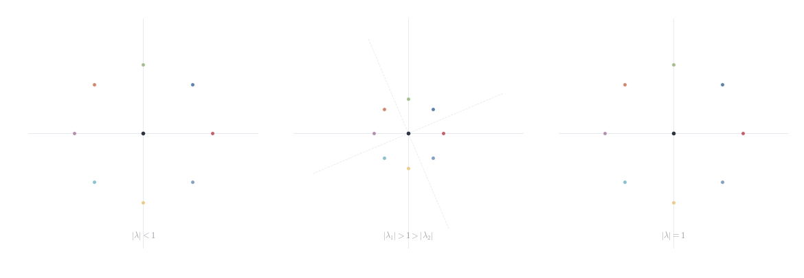
This is the key formula: the system decomposes into d independent scalar recurrences, one per eigendirection. The asymptotic behavior is controlled by the spectral radius \rho(A) = \max_{1 \le i \le d} |\lambda_i|.
(See Theorem 9.14 in Chapter 8 for the definition and key convergence criterion.)
Theorem 14.3 Let A \in M_d(\mathbb{C}) be diagonalizable. Then A^n \to 0 as n \to \infty if and only if \rho(A) < 1.
Proof. If \rho(A) < 1, then |\lambda_i| < 1 for all i, so \lambda_i^n \to 0. Since A^n = P D^n P^{-1}, we have \|A^n\| \le \|P\| \|P^{-1}\| \max_i |\lambda_i|^n \to 0.
Conversely, if some |\lambda_i| \ge 1, let v_i be a corresponding eigenvector. Then A^n v_i = \lambda_i^n v_i does not converge to 0, so A^n \not\to 0. \square
For non-diagonalizable matrices, the Jordan canonical form (Chapter 8, Section 9.8) shows that the same result holds: A^n \to 0 if and only if \rho(A) < 1. The Jordan blocks J_k(\lambda) = \lambda I + N contribute polynomial factors n^{k-1} that cannot overcome exponential decay when |\lambda| < 1. This is a good preview of why Jordan form matters: it handles exactly the cases where diagonalization fails.
14.2 Stability of Discrete Dynamical Systems
Consider the autonomous system x_{n+1} = A x_n, \quad x_0 \in \mathbb{F}^d, where A \in M_d(\mathbb{F}) is the evolution operator. A point x^* \in \mathbb{F}^d is an equilibrium if A x^* = x^*, equivalently (A - I)x^* = 0. The zero vector is always an equilibrium.
Definition 14.3 (Stability of equilibrium) The zero equilibrium of x_{n+1} = A x_n is:
Stable if for every \varepsilon > 0 there exists \delta > 0 such that \|x_0\| < \delta implies \|x_n\| < \varepsilon for all n \ge 0
Asymptotically stable if it is stable and additionally x_n \to 0 for all x_0 in a neighborhood of 0
Unstable if it is not stable
Theorem 14.4 Consider x_{n+1} = A x_n with A \in M_d(\mathbb{C}).
The zero equilibrium is asymptotically stable if and only if \rho(A) < 1
The zero equilibrium is unstable if \rho(A) > 1
If \rho(A) = 1 and A is diagonalizable with all eigenvalues on the unit circle simple, the system is stable but not asymptotically stable
Proof.
- Suppose \rho(A) < 1. By Theorem 14.3, A^n \to 0. Since A^n \to 0, the sequence (\|A^n\|) is convergent and hence bounded; let M := \sup_{n \ge 0} \|A^n\| < \infty. For any x_0, \|x_n\| = \|A^n x_0\| \le \|A^n\| \|x_0\| \le M \|x_0\|. Given \varepsilon > 0, take \delta = \varepsilon / M; then \|x_0\| < \delta implies \|x_n\| < \varepsilon for all n \ge 0, so the zero equilibrium is stable. Moreover x_n = A^n x_0 \to 0 for all x_0, so it is asymptotically stable.
Conversely, if \rho(A) \ge 1, there exists an eigenvalue \lambda with |\lambda| \ge 1 and eigenvector v \neq 0. Then A^n v = \lambda^n v, so \|A^n v\| = |\lambda|^n \|v\| \ge \|v\| > 0, and A^n v \not\to 0. Hence the zero equilibrium is not asymptotically stable.
If \rho(A) > 1, there exists \lambda with |\lambda| > 1. For the corresponding eigenvector v, we have \|A^n v\| = |\lambda|^n \|v\| \to \infty, so the system is unstable.
If \rho(A) = 1 and A is diagonalizable with all eigenvalues on the unit circle, the system is stable but not asymptotically stable (orbits remain bounded but do not decay). For non-diagonalizable matrices with \rho(A) = 1, Jordan blocks can introduce polynomial growth, leading to instability. \square
This theorem reduces the stability question to a spectral problem: compute eigenvalues and check |\lambda_i| < 1 for all i.
14.3 Predator–Prey Dynamics
The Lotka–Volterra model describes interaction between predators and prey. Let x_n denote prey population and y_n predator population at time n. The discrete-time linearization near an equilibrium yields \begin{pmatrix} x_{n+1} \\ y_{n+1} \end{pmatrix} = \begin{pmatrix} 1 + a & -b \\ c & 1 - d \end{pmatrix} \begin{pmatrix} x_n \\ y_n \end{pmatrix}, where a, b, c, d > 0 are parameters encoding growth rates, predation efficiency, and mortality. Stability of the equilibrium is determined by whether the eigenvalues of this 2 \times 2 matrix satisfy |\lambda| < 1.
The characteristic polynomial is \det(A - \lambda I) = \lambda^2 - (2 + a - d)\lambda + (1 + a)(1 - d) + bc. The continuous-time Lotka–Volterra model has purely imaginary eigenvalues at its positive equilibrium, indicating neutral stability and persistent oscillation. The discrete model inherits this marginal behavior: the eigenvalues of A near the equilibrium lie close to the unit circle, making the system sensitive to parameter values.
14.4 Stochastic Matrices and Probability Vectors
A matrix P \in M_d(\mathbb{R}) is column-stochastic if P_{ij} \ge 0 for all i, j and \sum_{i=1}^d P_{ij} = 1 \quad \text{for all } j.
Equivalently, \mathbf{1}^T P = \mathbf{1}^T where \mathbf{1} = (1, \ldots, 1)^T.
A vector x \in \mathbb{R}^d is a probability vector if x_i \ge 0 for all i and \sum_{i=1}^d x_i = 1.
Lemma 14.1 If P is column-stochastic and x is a probability vector, then Px is a probability vector.
Proof. Nonnegativity: (Px)_i = \sum_j P_{ij} x_j \ge 0 since P_{ij}, x_j \ge 0. Normalization: \sum_i (Px)_i = \sum_i \sum_j P_{ij} x_j = \sum_j x_j \sum_i P_{ij} = \sum_j x_j \cdot 1 = 1. \quad \square
Lemma 14.2 Every column-stochastic matrix has 1 as an eigenvalue.
Proof. Since \mathbf{1}^T P = \mathbf{1}^T, we have P^T \mathbf{1} = \mathbf{1}, so 1 is an eigenvalue of P^T. Since P and P^T share eigenvalues, 1 is an eigenvalue of P. \square
Definition 14.4 (Steady-state distribution) A vector \pi \in \mathbb{R}^d is a steady-state distribution for P if \pi is a probability vector and P\pi = \pi.
Existence is guaranteed by Lemma 14.2. Uniqueness requires additional hypotheses — specifically, that the chain is irreducible and aperiodic, as established below.
14.5 Markov Chains and Transition Matrices
Let (X_n)_{n=0}^\infty be a sequence of random variables taking values in a finite state space \mathcal{S} = \{1, \ldots, d\}. The sequence is a Markov chain if \mathbb{P}(X_{n+1} = j \mid X_n = i, X_{n-1}, \ldots, X_0) = \mathbb{P}(X_{n+1} = j \mid X_n = i) for all n \ge 0 and all states i, j \in \mathcal{S}. This is the Markov property: the future depends on the present but not the past. Given where you are now, knowing how you got there provides no additional predictive information.
The transition probabilities P_{ij} = \mathbb{P}(X_{n+1} = j \mid X_n = i) form the transition matrix P = (P_{ij}), which in the probabilistic convention is row-stochastic: P_{ij} \ge 0 and \sum_j P_{ij} = 1.
Convention. We adopt the column-stochastic convention throughout: we redefine P_{ij} = \mathbb{P}(X_{n+1} = i \mid X_n = j), so column j of P is the distribution of the next state given current state j. This ensures the state evolution is x^{(n+1)} = Px^{(n)}, making the connection to matrix powers and eigenvalue theory transparent. Let x^{(n)} \in \mathbb{R}^d denote the distribution at time n with x_i^{(n)} = \mathbb{P}(X_n = i). Then x^{(n+1)} = P x^{(n)}.
Iterating gives x^{(n)} = P^n x^{(0)} for any initial distribution x^{(0)}.
Definition 14.5 (Irreducibility) A Markov chain with transition matrix P is irreducible if for every pair of states i, j \in \mathcal{S}, there exists n \ge 0 such that (P^n)_{ij} > 0.
Irreducibility means every state is accessible from every other state. Graphically, the directed graph with adjacency matrix P is strongly connected. Without irreducibility, the chain can get “trapped” in a subset of states.
Definition 14.6 (Aperiodicity) The period of state i is d_i = \gcd\{n \ge 1 : (P^n)_{ii} > 0\}. The chain is aperiodic if d_i = 1 for all i.
Periodicity arises when states are partitioned into cycles. For instance, a bipartite graph induces period 2: the walker alternates between vertex sets. Aperiodicity ensures eventual return to every state at arbitrary times, not just multiples of the period.

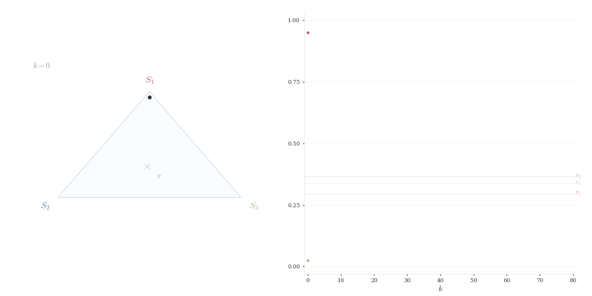
Theorem 14.5 Let P be a column-stochastic matrix corresponding to an irreducible, aperiodic Markov chain. Then:
There exists a unique probability vector \pi with P\pi = \pi and \pi_i > 0 for all i
For any initial distribution x^{(0)}, we have \lim_{n \to \infty} P^n x^{(0)} = \pi
The convergence is exponential: there exist constants C > 0 and \lambda \in (0, 1) such that \|P^n x^{(0)} - \pi\| \le C \lambda^n.
This result follows from the Perron–Frobenius theorem, established in the next section. The steady state \pi represents the long-run proportion of time spent in each state — regardless of where the chain starts, it eventually “forgets” its initial condition.
14.5.1 Example: Gambler’s Ruin
A gambler starts with k dollars and plays a fair game: each round, she wins 1 dollar with probability p or loses 1 dollar with probability q = 1 - p. The game ends when she reaches 0 (ruin) or N (target). Let X_n denote her fortune at time n. This is a Markov chain on \{0, 1, \ldots, N\} with transition matrix P_{i,i+1} = p, \quad P_{i,i-1} = q \quad \text{for } 1 \le i \le N-1, and absorbing states P_{0,0} = P_{N,N} = 1.
The probability of reaching N before 0 starting from k satisfies the recurrence u_k = p u_{k+1} + q u_{k-1}, \quad u_0 = 0, \quad u_N = 1.
For p \neq q, the solution is u_k = \frac{1 - (q/p)^k}{1 - (q/p)^N}.
For p = q = 1/2 (fair game), u_k = k/N. The formula reflects the geometric sequence structure of the eigenvalues of the tridiagonal transition matrix restricted to transient states: the characteristic decay rate q/p is precisely the ratio of the two relevant eigenvalues, and the boundary conditions select the unique linear combination satisfying u_0 = 0, u_N = 1.
14.6 The Perron–Frobenius Theorem
We state the Perron–Frobenius theorem for non-negative matrices, the foundation for analyzing stochastic systems.
Theorem 14.6 (Perron–Frobenius theorem) Let A \in M_d(\mathbb{R}) satisfy A_{ij} \ge 0 for all i, j. Assume A is irreducible: for every i, j, there exists k \ge 1 such that (A^k)_{ij} > 0.
Then:
A has a positive real eigenvalue r = \rho(A) where \rho(A) = \max\{|\lambda| : \lambda \text{ eigenvalue of } A\} is the spectral radius
r has algebraic and geometric multiplicity 1
There exists an eigenvector v > 0 (meaning v_i > 0 for all i) such that Av = rv
Any other eigenvalue \lambda satisfies |\lambda| < r, provided A is aperiodic in the sense that \gcd\{k \ge 1 : (A^k)_{ii} > 0\} = 1 for all i
The full proof of the Perron–Frobenius theorem requires tools from topology and functional analysis that lie beyond this course:
- Brouwer fixed-point theorem: Every continuous map from a compact convex set to itself has a fixed point
- Compactness arguments: The set of probability vectors is compact in \mathbb{R}^d
- Positive operator theory: Properties of linear maps that preserve the positive cone
These belong to a graduate course in functional analysis or operator theory. We accept the theorem and apply its consequences.
Proof. Omitted. See Perron (1907) and Frobenius (1912) for the original proofs. \square
Corollary 14.1 Let P be column-stochastic, irreducible, and aperiodic. Then:
There exists a unique probability vector \pi with P\pi = \pi
All components of \pi are strictly positive
For any probability vector x, \lim_{n \to \infty} P^n x = \pi
Proof. By Theorem 14.6 applied to P, the eigenvalue r = 1 (from Lemma 14.2) is simple with positive eigenvector v. Normalize \pi = v / \|v\|_1 to obtain a probability vector. Uniqueness follows from simplicity of r = 1.
For (c), decompose x = c\pi + w where w lies in the span of the remaining eigenvectors. The component w decays exponentially since all other eigenvalues satisfy |\lambda| < 1 by aperiodicity. \square
This result underlies the convergence of Markov chain Monte Carlo methods, the PageRank algorithm, and equilibrium distributions in statistical mechanics.
14.7 Continuous-Time Systems and the Matrix Exponential
A continuous-time linear system is \frac{dx}{dt} = B x, \quad x(0) = x_0 \in \mathbb{F}^d, where B \in M_d(\mathbb{F}). The solution is x(t) = e^{Bt} x_0 where the matrix exponential e^{Bt} is defined by the power series (see Chapter 8, Section 9.9): e^{Bt} = \sum_{k=0}^\infty \frac{(Bt)^k}{k!} = I + Bt + \frac{(Bt)^2}{2!} + \cdots.
Theorem 14.7 For B \in M_d(\mathbb{C}):
The series defining e^{Bt} converges absolutely for all t \in \mathbb{R}
\frac{d}{dt} e^{Bt} = B e^{Bt} = e^{Bt} B
If B = P D P^{-1} is diagonalizable, then e^{Bt} = P e^{Dt} P^{-1} where e^{Dt} = \operatorname{diag}(e^{\lambda_1 t}, \ldots, e^{\lambda_d t})
e^{B(t+s)} = e^{Bt} e^{Bs} for all t, s \in \mathbb{R}
These properties are proved in Chapter 8, Section 9.9. The key tool is that submultiplicative matrix norms ensure absolute convergence of the series.
Theorem 14.8 The system \frac{dx}{dt} = Bx satisfies x(t) \to 0 as t \to \infty for all x_0 if and only if \operatorname{Re}(\lambda) < 0 for all eigenvalues \lambda of B.
Proof. If B = PDP^{-1}, then e^{Bt} = P e^{Dt} P^{-1} with e^{Dt} = \operatorname{diag}(e^{\lambda_1 t}, \ldots, e^{\lambda_d t}). Since |e^{\lambda t}| = e^{\operatorname{Re}(\lambda) t}, we have e^{\lambda t} \to 0 iff \operatorname{Re}(\lambda) < 0. \square
The parallel with discrete-time stability is clean: discrete requires |\lambda| < 1 (eigenvalues inside the unit disk); continuous requires \operatorname{Re}(\lambda) < 0 (eigenvalues in the left half-plane).
14.7.1 Connection to Discrete Systems
Discretizing \frac{dx}{dt} = Bx via Euler’s method with step \Delta t gives A = I + \Delta t B; an eigenvalue \mu of B becomes \lambda = 1 + \Delta t \mu for A, so negative real part (continuous stability) maps to |\lambda| < 1 (discrete stability) for small \Delta t.
14.8 Closing Remarks
The long-run behavior of x_{n+1} = Ax_n reduces to a spectral question: eigenvalues inside the unit disk give decay, outside give growth, on the circle give oscillation. Diagonalization makes this explicit — the trajectory decomposes into d independent scalar recurrences c_i \lambda_i^n v_i, and the spectral radius \rho(A) is the decisive quantity.
Stochastic matrices instantiate this: the Perron–Frobenius theorem guarantees a unique positive steady state for irreducible aperiodic chains, and convergence to it is exponential with rate |\lambda_2|. The continuous-time parallel — \frac{dx}{dt} = Bx stable iff \operatorname{Re}(\lambda) < 0 — is the same story with the unit disk replaced by the left half-plane.