6 Higher-Order Derivatives
Chapter 3 defined the total derivative Df_a and identified its entries as partial derivatives. What it left open is the question of when partial derivatives are enough to guarantee differentiability — the converse direction. The answer, C^1 implies differentiable, is the first theorem here. After that we go to second order: differentiating Df to get D^2f, proving that mixed partial derivatives commute for C^2 functions, and assembling everything into Taylor’s theorem in \mathbb{R}^n.
The payoff is a clean picture: near a point a, a smooth function looks like a polynomial in the displacement h, with coefficients given by its derivatives at a. That polynomial is the Taylor expansion, and understanding it — particularly its second-order term — is the foundation for the optimisation theory of Chapter 6.
6.1 When Partial Derivatives Are Enough
Partial derivatives probe f only along coordinate directions, while differentiability requires a uniform approximation in all directions at once. The gap between them is real: as we saw in Chapter 3, a function can have all partial derivatives at a point without being differentiable, or even continuous, there. But if the partial derivatives not only exist but vary continuously, the gap closes.
Theorem 6.1 (C^1 implies differentiable) If all partial derivatives \partial_j f_i exist and are continuous on U, then f is differentiable on U, and Df_a has matrix J_f(a).
Proof. Fix a \in U and h = \sum_j h_j e_j small. Write the telescoping sum f(a+h) - f(a) = \sum_{j=1}^n \bigl[f(a + h_1 e_1 + \cdots + h_j e_j) - f(a + h_1 e_1 + \cdots + h_{j-1} e_{j-1})\bigr]. Each term changes only the j-th coordinate, so the single-variable mean value theorem gives a point \xi_j — on the segment between a + h_1 e_1 + \cdots + h_{j-1}e_{j-1} and the next step — with f(a + h_1 e_1 + \cdots + h_j e_j) - f(a + h_1 e_1 + \cdots + h_{j-1} e_{j-1}) = \partial_j f(\xi_j)\, h_j. So f(a+h) - f(a) = \sum_j \partial_j f(\xi_j)\, h_j. Subtracting the candidate linear approximation J_f(a)h = \sum_j \partial_j f(a)\, h_j: \frac{\|f(a+h) - f(a) - J_f(a)h\|}{\|h\|} \leq \sum_{j=1}^n \|\partial_j f(\xi_j) - \partial_j f(a)\| \cdot \frac{|h_j|}{\|h\|}. Each ratio |h_j|/\|h\| \leq 1. As h \to 0 each \xi_j \to a, and continuity of the partial derivatives gives \|\partial_j f(\xi_j) - \partial_j f(a)\| \to 0. \square
The proof is a good illustration of why the telescoping idea works: each step changes only one coordinate, so the single-variable mean value theorem applies, and continuity of the partial derivatives makes each correction term small.
In practice this is how differentiability is verified: compute the partial derivatives and check they are continuous. If they are, you have C^1, which gives differentiability for free.
6.2 Higher Derivatives
If f : U \to \mathbb{R}^m is differentiable on U, the map Df : U \to \mathscr{L}(\mathbb{R}^n, \mathbb{R}^m) sends each point a to the linear map Df_a. The space \mathscr{L}(\mathbb{R}^n, \mathbb{R}^m) of linear maps \mathbb{R}^n \to \mathbb{R}^m is itself a finite-dimensional vector space — it is isomorphic to the space of m \times n matrices, hence to \mathbb{R}^{mn}. So we can ask whether Df is itself differentiable.
Definition 6.1 (Second derivative) If Df : U \to \mathscr{L}(\mathbb{R}^n, \mathbb{R}^m) is differentiable at a, its total derivative is the second derivative D^2f_a, a linear map D^2f_a : \mathbb{R}^n \to \mathscr{L}(\mathbb{R}^n, \mathbb{R}^m). Equivalently, D^2f_a is a bilinear map \mathbb{R}^n \times \mathbb{R}^n \to \mathbb{R}^m via (v, w) \mapsto D^2f_a(v)(w).
The second derivative measures how Df changes as the basepoint moves. For a scalar function f : U \to \mathbb{R}, it is a bilinear form \mathbb{R}^n \times \mathbb{R}^n \to \mathbb{R}. Whether this form is symmetric — D^2f_a(v,w) = D^2f_a(w,v) — is not part of the definition; it is a theorem, proved in the next section.
Higher derivatives are defined inductively: D^k f_a is the total derivative of D^{k-1}f, a k-linear map (\mathbb{R}^n)^k \to \mathbb{R}^m. A map is C^k if D^k f exists and is continuous, and smooth if C^k for all k.
6.3 Clairaut’s Theorem
The second derivative, as a bilinear form, has entries \partial_i \partial_j f(a) — differentiating first in the j-th direction and then in the i-th. In principle the order could matter: \partial_i \partial_j f and \partial_j \partial_i f are defined by different limiting processes. For C^2 functions they agree.
Theorem 6.2 (Clairaut’s theorem) If f \in C^2(U), then \partial_i \partial_j f = \partial_j \partial_i f on U for all i, j.
Proof. Fix a and consider small s, t. Define the second difference \Delta(s,t) = f(a + se_i + te_j) - f(a + se_i) - f(a + te_j) + f(a). Set \varphi(s) = f(a + se_i + te_j) - f(a + se_i). The mean value theorem applied to \varphi on [0,s] gives some s^* with \Delta(s,t) = \varphi'(s^*) \cdot s = (\partial_i f(a + s^* e_i + te_j) - \partial_i f(a + s^* e_i)) \cdot s. Applying the mean value theorem again to the expression in parentheses, as a function of t on [0,t], gives some t^* with \Delta(s,t) = st\, \partial_j \partial_i f(a + s^* e_i + t^* e_j). The same calculation with the roles of i and j swapped gives \Delta(s,t) = st\, \partial_i \partial_j f(a + s^{**} e_j + t^{**} e_i). Both expressions equal \Delta(s,t). Divide by st, let s, t \to 0: both a + s^* e_i + t^* e_j and a + s^{**} e_j + t^{**} e_i approach a, and continuity of the second partial derivatives gives \partial_j \partial_i f(a) = \partial_i \partial_j f(a). \square
This says D^2f_a is a symmetric bilinear form whenever f \in C^2. The hypothesis is necessary: without continuity of the second partial derivatives, the mixed partials can genuinely differ at a point.
6.4 The Hessian
For a scalar function f : U \to \mathbb{R}, the second derivative D^2f_a is a symmetric bilinear form on \mathbb{R}^n. Its matrix in the standard basis is the Hessian.
Definition 6.2 (Hessian) The Hessian of f \in C^2(U) at a is the symmetric n \times n matrix H_f(a) = \bigl[\partial_i \partial_j f(a)\bigr]_{1 \leq i,j \leq n}.
Symmetry of H_f(a) is Clairaut’s theorem. Since H_f(a) is real and symmetric, the spectral theorem from linear algebra applies: it has n real eigenvalues \lambda_1 \leq \cdots \leq \lambda_n and an orthonormal eigenbasis. In that eigenbasis, h^T H_f(a)\, h = \sum_{i=1}^n \lambda_i c_i^2 where c_i = \langle h, v_i \rangle are the coordinates of h. Whether this sum is always positive, always negative, or can have either sign depends entirely on the signs of the eigenvalues — and this is what controls whether a is a local minimum, maximum, or saddle. That analysis is Chapter 6.
Example. For f(x,y,z) = x^2 + 2xy + y^2 + z^4 at a = 0: H_f(0) = \begin{pmatrix} 2 & 2 & 0 \\ 2 & 2 & 0 \\ 0 & 0 & 0 \end{pmatrix}. The eigenvalues are 0, 0, 4. The Hessian is positive semidefinite — the z-direction and the direction x = -y are both flat to second order. Whether 0 is a local minimum requires looking at higher-order terms.
6.5 Taylor’s Theorem
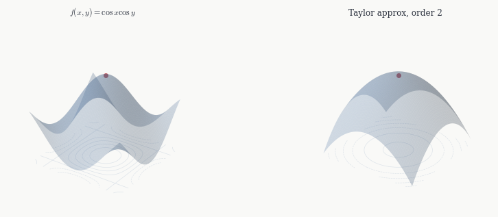
In single-variable calculus, Taylor’s theorem says a C^k function near a looks like a degree-k polynomial in h = x - a: f(a + h) = f(a) + f'(a)h + \frac{f''(a)}{2}h^2 + \cdots + \frac{f^{(k)}(a)}{k!}h^k + o(h^k). In \mathbb{R}^n the same thing is true, with h \in \mathbb{R}^n and polynomial now meaning a polynomial in the components h_1, \ldots, h_n.
Theorem 6.3 (Taylor’s theorem) Let f \in C^k(U) with U \subset \mathbb{R}^n convex. For a \in U and h with a + h \in U: f(a+h) = f(a) + Df_a(h) + \frac{1}{2} D^2f_a(h,h) + \cdots + \frac{1}{k!} D^kf_a(h, \ldots, h) + o(\|h\|^k).
Proof. Set g(t) = f(a + th) for t \in [0,1]. This is a single-variable C^k function on [0,1], and g(1) = f(a+h), g(0) = f(a). The chain rule gives g'(t) = Df_{a+th}(h), and differentiating again g''(t) = D^2f_{a+th}(h,h), and so on: g^{(j)}(t) = D^jf_{a+th}(h, \ldots, h). Apply the single-variable Taylor theorem to g at t = 0 and evaluate at t = 1. \square
The key step — that g^{(j)}(t) = D^j f_{a+th}(h,\ldots,h) — is just the chain rule applied j times. The j-th term in the expansion, \frac{1}{j!} D^j f_a(h,\ldots,h), is a degree-j polynomial in h when expanded in coordinates. The first two terms are familiar: Df_a(h) = \nabla f(a) \cdot h (the directional derivative) and \frac{1}{2}D^2f_a(h,h) = \frac{1}{2} h^T H_f(a)\, h (the Hessian quadratic form). Together:
Theorem 6.4 (Second-order Taylor) If f \in C^2(U): f(a+h) = f(a) + \nabla f(a) \cdot h + \frac{1}{2}\, h^T H_f(a)\, h + o(\|h\|^2).
At a critical point where \nabla f(a) = 0, the linear term vanishes and the Hessian quadratic form is the leading term. This is why the Hessian controls the local behaviour at critical points.
6.6 Multi-Index Notation
Writing general k-th order terms explicitly becomes impractical fast: a function of n variables has \binom{n+k-1}{k} distinct partial derivatives of order k. For n = 3, k = 3, that is already ten. Multi-index notation packages all of them into the same form as the one-variable case.
Definition 6.3 (Multi-index) A multi-index \alpha = (\alpha_1, \ldots, \alpha_n) \in \mathbb{Z}_{\geq 0}^n has order |\alpha| = \alpha_1 + \cdots + \alpha_n. We write \alpha! = \alpha_1!\cdots\alpha_n!, \qquad h^\alpha = h_1^{\alpha_1}\cdots h_n^{\alpha_n}, \qquad \partial^\alpha = \partial_1^{\alpha_1}\cdots\partial_n^{\alpha_n}.
With this notation, D^k f_a(h, \ldots, h) expands in coordinates as D^k f_a(h, \ldots, h) = \sum_{|\alpha|=k} \frac{k!}{\alpha!}\, (\partial^\alpha f(a))\, h^\alpha, by the multinomial theorem. Substituting into Taylor’s theorem:
Theorem 6.5 (Taylor’s theorem (multi-index form)) If f \in C^k(U) with U convex: f(a+h) = \sum_{|\alpha| \leq k} \frac{\partial^\alpha f(a)}{\alpha!}\,h^\alpha + o(\|h\|^k).
This is exactly the single-variable Taylor formula with \alpha! replacing k! and h^\alpha replacing h^k. For n = 1 it reduces to it literally.
Example. For f : \mathbb{R}^2 \to \mathbb{R} with k = 2, the multi-indices of order \leq 2 are (0,0), (1,0), (0,1), (2,0), (1,1), (0,2). The expansion is f(a+h) = f(a) + \partial_1 f(a)\,h_1 + \partial_2 f(a)\,h_2 + \frac{1}{2}\partial_1^2 f(a)\,h_1^2 + \partial_1\partial_2 f(a)\,h_1 h_2 + \frac{1}{2}\partial_2^2 f(a)\,h_2^2 + o(\|h\|^2). The h_1 h_2 term has coefficient \partial_1\partial_2 f(a) rather than \frac{1}{2}\partial_1\partial_2 f(a) because the multi-index (1,1) has \alpha! = 1, while the Hessian matrix entry [H_f]_{12} accounts for both the (1,1) and (1,1)-transposed contributions.