12 Green’s Theorem
The fundamental theorem of calculus says that the integral of a derivative over an interval recovers the values at the endpoints: \int_a^b f'(x)\, dx = f(b) - f(a). The interval has a boundary — two points — and f(b) - f(a) is the integral of f over that boundary, with signs determined by orientation. Green’s theorem is the two-dimensional version of this: the integral of a certain derivative over a region \Omega \subset \mathbb{R}^2 equals an integral over its boundary curve \partial\Omega. The region is one dimension higher than the interval, the boundary is one dimension higher than the endpoints, and the derivative that appears is a combination of partial derivatives in two variables.
What makes Green’s theorem more than just an analogy is that the proof is essentially the same: apply the fundamental theorem of calculus in each coordinate direction and observe that the interior terms cancel, leaving only boundary contributions. The calculation is completely explicit, and seeing it once makes the mechanism of all the integral theorems — Green, Stokes, the Divergence theorem — transparent.
12.1 The Theorem
We need a class of regions whose boundaries are smooth enough to integrate over. A Jordan domain \Omega \subset \mathbb{R}^2 is a bounded open set whose boundary \partial\Omega is a finite union of simple closed C^1 curves. The orientation of \partial\Omega is the positive orientation: traversing the boundary with the interior of \Omega on the left. For a convex region this is counterclockwise; for a region with holes, the outer boundary runs counterclockwise and each inner boundary (around a hole) runs clockwise.
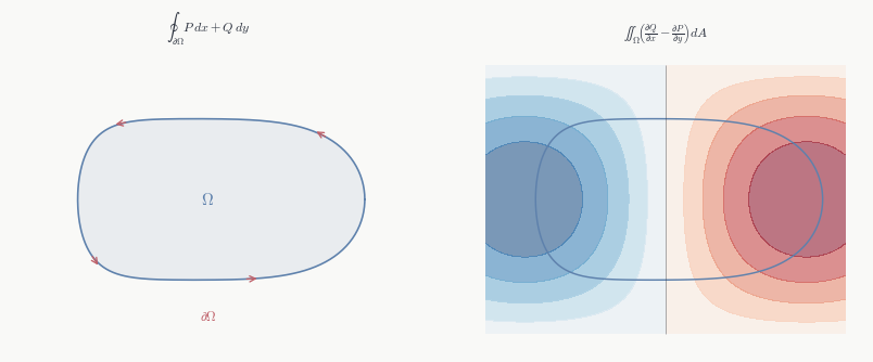
Theorem 12.1 (Green’s theorem) Let \Omega \subset \mathbb{R}^2 be a Jordan domain and P, Q : \overline\Omega \to \mathbb{R} be C^1 functions. Then \oint_{\partial\Omega} P\, dx + Q\, dy = \iint_\Omega \left(\frac{\partial Q}{\partial x} - \frac{\partial P}{\partial y}\right) dA.
Before the proof it is worth pausing on what the two sides are. The left side is the line integral of the vector field F = (P, Q) around the boundary of \Omega — it measures circulation. The right side integrates the scalar \partial_x Q - \partial_y P over the interior — this is the curl of F in two dimensions, the infinitesimal rotation of F at each point. Green’s theorem says: the total circulation around the boundary equals the total rotation inside. This is not obvious, but once you see the proof it is hard to imagine it being otherwise.
Proof. It suffices to prove the two identities \oint_{\partial\Omega} P\, dx = -\iint_\Omega \frac{\partial P}{\partial y}\, dA \qquad \text{and} \qquad \oint_{\partial\Omega} Q\, dy = \iint_\Omega \frac{\partial Q}{\partial x}\, dA separately and add them. We prove the first; the second is identical with P and Q swapped and the sign adjusted.
First suppose \Omega is a vertically simple region: \Omega = \{(x,y): a \leq x \leq b,\; \phi(x) \leq y \leq \psi(x)\} for continuous \phi \leq \psi. Then by Theorem 10.2 and the fundamental theorem in y: -\iint_\Omega \frac{\partial P}{\partial y}\, dA = -\int_a^b \int_{\phi(x)}^{\psi(x)} \frac{\partial P}{\partial y}(x,y)\, dy\, dx = -\int_a^b \bigl[P(x,\psi(x)) - P(x,\phi(x))\bigr]\, dx. The boundary \partial\Omega consists of four pieces: the bottom curve y = \phi(x) traversed left to right, the right vertical segment, the top curve y = \psi(x) traversed right to left, and the left vertical segment. On the vertical segments dx = 0 so they contribute nothing. The bottom contributes \int_a^b P(x,\phi(x))\, dx and the top contributes -\int_a^b P(x,\psi(x))\, dx (the minus sign from traversing right to left). Together: \oint_{\partial\Omega} P\, dx = \int_a^b P(x,\phi(x))\, dx - \int_a^b P(x,\psi(x))\, dx = -\int_a^b \bigl[P(x,\psi(x)) - P(x,\phi(x))\bigr]\, dx. This matches the interior integral. For a general Jordan domain, subdivide \Omega into finitely many vertically simple pieces, apply the result to each, and observe that interior boundary segments between adjacent pieces are traversed in opposite directions and cancel. \square
12.2 Consequences and Applications
12.2.1 The area formula
Setting P = 0 and Q = x in Green’s theorem: \oint_{\partial\Omega} x\, dy = \iint_\Omega 1\, dA = \operatorname{Area}(\Omega). Similarly P = -y, Q = 0 gives \oint_{\partial\Omega} -y\, dx = \operatorname{Area}(\Omega). Averaging: \operatorname{Area}(\Omega) = \frac{1}{2}\oint_{\partial\Omega} x\, dy - y\, dx. This is a remarkable formula: the area of a region is determined entirely by a line integral around its boundary, with no reference to the interior. For a polygon with vertices (x_0, y_0), \ldots, (x_{n-1}, y_{n-1}) it gives the shoelace formula \operatorname{Area} = \frac{1}{2}\left|\sum_{i=0}^{n-1} (x_i y_{i+1} - x_{i+1} y_i)\right|, where indices are taken mod n. This is the formula used in GIS software to compute areas of polygons on maps.
12.2.2 Conservative fields revisited
Green’s theorem gives an independent proof of the converse direction in the conservative fields theorem from Chapter 9, for the special case of \mathbb{R}^2.
If \operatorname{curl} F = \partial_x Q - \partial_y P = 0 on a simply connected domain U \subset \mathbb{R}^2, then for any closed curve \gamma in U bounding a region \Omega \subset U: \oint_\gamma P\, dx + Q\, dy = \iint_\Omega \left(\frac{\partial Q}{\partial x} - \frac{\partial P}{\partial y}\right) dA = 0. Since every closed curve in a simply connected domain bounds such a region, every closed line integral vanishes. By Theorem 11.1 (from Chapter 9), F is conservative.
This is the argument that was deferred in Chapter 9: Stokes’ theorem is the general version of this reasoning, and Green’s theorem is its incarnation in two dimensions.
12.2.3 Green’s identities
Let u, v : \overline\Omega \to \mathbb{R} be C^2. Taking F = u\nabla v in the divergence theorem (which in two dimensions is just Green’s theorem applied to the appropriate components): \iint_\Omega u\, \Delta v\, dA = \oint_{\partial\Omega} u\, \frac{\partial v}{\partial n}\, ds - \iint_\Omega \nabla u \cdot \nabla v\, dA, where \partial v/\partial n = \nabla v \cdot \hat n is the outward normal derivative of v on \partial\Omega. This is Green’s first identity. Swapping u and v and subtracting gives Green’s second identity: \iint_\Omega (u\,\Delta v - v\,\Delta u)\, dA = \oint_{\partial\Omega} \left(u\,\frac{\partial v}{\partial n} - v\,\frac{\partial u}{\partial n}\right) ds. These identities are fundamental in the theory of partial differential equations. If u is harmonic (\Delta u = 0), Green’s second identity with v = 1 gives \oint_{\partial\Omega} \partial u/\partial n\, ds = 0: the total outward flux of a harmonic function through any closed curve is zero. If both u and v are harmonic, the right side must be symmetric in u and v, reflecting the self-adjointness of the Laplacian.
12.3 The Geometric Picture
It is worth understanding Green’s theorem geometrically, not just as a calculation. The quantity \partial_x Q - \partial_y P is the two-dimensional curl of (P,Q) — the infinitesimal circulation of the field per unit area at a point. Green’s theorem says the global circulation around \partial\Omega is the total of all the infinitesimal circulations inside \Omega.
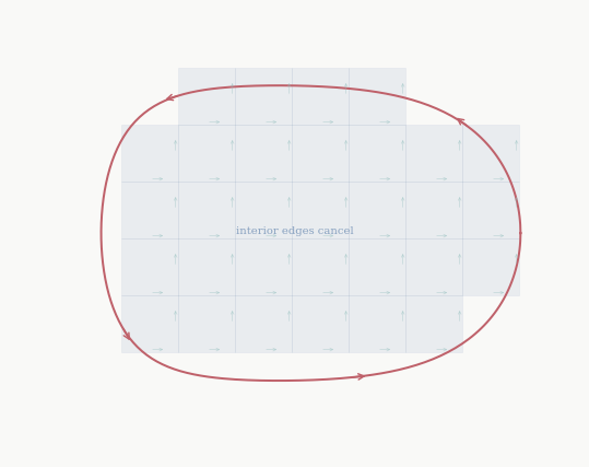
Why should these be equal? Consider tiling \Omega with tiny squares. The circulation of F around each tiny square is approximately (\partial_x Q - \partial_y P) \cdot \text{area}. When we sum over all squares, the contributions from interior edges cancel: each interior edge is shared by two adjacent squares and traversed in opposite directions. Only the edges on \partial\Omega survive. The sum of circulations over all tiny squares is therefore the circulation around the outer boundary.
This telescoping cancellation is the same mechanism as in the proof — the interior boundary pieces cancel when we subdivide into simple regions — and it is the same mechanism as in the fundamental theorem of calculus itself, where interior contributions cancel and only the endpoints remain. In all dimensions and in all versions, this is what an integral theorem is.
12.4 Relationship to the Other Integral Theorems
Green’s theorem is the n = 2 case of a single general theorem. Writing it in vector field notation, with F = (P, Q): \oint_{\partial\Omega} F \cdot d\gamma = \iint_\Omega (\nabla \times F) \cdot \hat k\, dA, where \hat k = (0,0,1) is the unit normal to the xy-plane and \nabla \times F = \partial_x Q - \partial_y P is the z-component of the three-dimensional curl. This is exactly Stokes’ theorem — applied to a flat surface in \mathbb{R}^3.
The Divergence theorem in two dimensions is Green’s theorem with F replaced by its 90° rotation (P,Q) \mapsto (-Q, P): the circulation of (-Q,P) around \partial\Omega equals the flux of F = (P,Q) outward through \partial\Omega, and \partial_x(-Q) + \partial_y P = -(\partial_x Q - \partial_y P) from the standard formula… actually one writes it directly as: if \hat n is the outward unit normal to \partial\Omega, \oint_{\partial\Omega} F \cdot \hat n\, ds = \iint_\Omega \nabla \cdot F\, dA. This is the two-dimensional divergence theorem, which follows immediately from Green’s theorem by rotating F by 90°.
So one theorem — Green’s — contains both Stokes and the Divergence theorem in two dimensions as special cases, depending on whether we contract F against the tangent or the normal of the boundary. In three dimensions, Stokes’ theorem handles surfaces and the Divergence theorem handles volumes, and they are genuinely different. But in two dimensions they are the same theorem, seen from two angles.