7 Vector Fields, Gradient, Divergence, and Curl

So far we have differentiated scalar fields f : U \to \mathbb{R}. The total derivative Df_a is a linear functional, the Hessian is a bilinear form, and the gradient is the vector that represents Df_a via the inner product. Now we want to differentiate vector fields — smooth maps F : U \to \mathbb{R}^n that assign a vector to each point. The velocity of a fluid, the force exerted by a magnetic field, the gradient of a temperature distribution: all of these are vector fields, and all of them can be differentiated.

The total derivative of a vector field F at a is DF_a : \mathbb{R}^n \to \mathbb{R}^n, a linear endomorphism — a square matrix in coordinates. This is richer than the scalar case, because a square matrix is not just a number: it has a trace, a symmetric part, an antisymmetric part, a determinant. The classical operations of vector calculus — divergence and curl — turn out to be exactly the trace and antisymmetric part of this matrix. They are not independent inventions; they are the natural decomposition of DF_a into its irreducible pieces.

This perspective makes the vector calculus identities transparent. The identity \operatorname{curl}(\nabla f) = 0 says the Hessian of a C^2 function is symmetric — that is Theorem 6.2. The identity \operatorname{div}(\operatorname{curl} F) = 0 says a certain antisymmetric matrix has zero trace — which is true for any antisymmetric matrix. Once you see this, none of these identities feel like facts to memorise; they feel like observations about matrices.

7.1 The Gradient

For a scalar field f : U \to \mathbb{R}, the total derivative Df_a : \mathbb{R}^n \to \mathbb{R} is a linear functional — an element of the dual space (\mathbb{R}^n)^*. From Chapter 1.5 we know that every linear functional on \mathbb{R}^n is given by an inner product with a unique vector. Applied here:

Definition 7.1 (Gradient) The gradient of f : U \to \mathbb{R} at a is the unique vector \nabla f(a) \in \mathbb{R}^n satisfying Df_a(v) = \langle \nabla f(a),\, v \rangle \qquad \text{for all } v \in \mathbb{R}^n. In standard coordinates, \nabla f(a) = (\partial_1 f(a), \ldots, \partial_n f(a))^T.

The gradient is the Riesz representative of the total derivative. The row vector J_f(a) = (\partial_1 f(a), \ldots, \partial_n f(a)) and the column vector \nabla f(a) contain the same entries — they differ only in how they act: J_f(a) acts by left-multiplication on column vectors, \nabla f(a) acts by inner product. In coordinates they look the same; the distinction matters when the inner product is not the standard one, as on a curved surface.

Two geometric facts follow immediately from this definition.

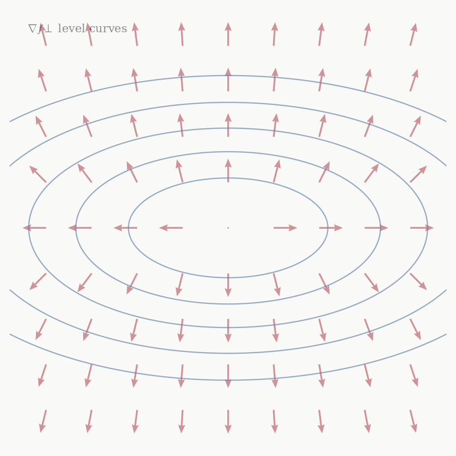
Theorem 7.1 (Gradient and level sets) Let f \in C^1(U) and \nabla f(a) \neq 0.

\nabla f(a) is perpendicular to the level set f^{-1}(f(a)): for every smooth curve \gamma in f^{-1}(f(a)) through a, \langle \nabla f(a), \gamma'(0) \rangle = 0.
\nabla f(a) points in the direction of steepest increase of f: among all unit vectors v, the directional derivative D_v f(a) = \langle \nabla f(a), v \rangle is maximised by v = \nabla f(a)/\|\nabla f(a)\|, with maximum value \|\nabla f(a)\|.

Proof. (i) The curve \gamma lies in f^{-1}(f(a)), so f(\gamma(t)) = f(a) for all t. Differentiating at t = 0 by the chain rule: Df_a(\gamma'(0)) = 0, which is \langle \nabla f(a), \gamma'(0)\rangle = 0.

Cauchy–Schwarz: \langle \nabla f(a), v \rangle \leq \|\nabla f(a)\| \|v\| = \|\nabla f(a)\|, with equality iff v is parallel to \nabla f(a). \square

Both parts say the same thing in different words: the Riesz representative of a nonzero linear functional is perpendicular to the functional’s kernel and points in the direction the functional increases fastest. Here the functional is Df_a, its kernel is the tangent hyperplane to the level set, and its Riesz representative is \nabla f(a). This is the geometric content of the gradient — not a formula, but the fact that it is the normal direction to the level set, scaled by the rate of change.

7.2 Divergence

For a vector field F : U \to \mathbb{R}^n, the total derivative DF_a : \mathbb{R}^n \to \mathbb{R}^n is a linear endomorphism — a square matrix in coordinates. A square matrix has several natural invariants. The simplest is its trace, which is basis-independent: \operatorname{tr}(SAS^{-1}) = \operatorname{tr}(A) for any invertible S, by the cyclic property \operatorname{tr}(AB) = \operatorname{tr}(BA).

Definition 7.2 (Divergence) The divergence of F : U \to \mathbb{R}^n is \operatorname{div} F(a) = \nabla \cdot F(a) = \operatorname{tr}(J_F(a)) = \sum_{i=1}^n \partial_i F_i(a).

Why the trace? The determinant of a linear map measures how it scales volumes. Near the identity, \det(I + tA) = 1 + t\operatorname{tr}(A) + O(t^2), so the trace is the infinitesimal rate of volume change. A vector field F generates a flow — the solutions to \dot{x} = F(x) — and the divergence measures how much that flow compresses or expands small volumes near a. Positive divergence: the flow is spreading out, like a source. Negative divergence: the flow is converging, like a sink. Zero divergence: the flow preserves volumes, like an incompressible fluid.

This interpretation also explains the notation \nabla \cdot F: it is the trace of the Jacobian, and it behaves formally like a dot product of the operator \nabla = (\partial_1, \ldots, \partial_n)^T with the vector field F = (F_1, \ldots, F_n)^T. The notation is a mnemonic, not a literal dot product — \nabla is an operator, not a vector.

7.3 Curl

In \mathbb{R}^n, the Jacobian J_F(a) is an n \times n matrix. Any square matrix decomposes uniquely into its symmetric and antisymmetric parts: J_F(a) = \underbrace{\tfrac{1}{2}(J_F + J_F^T)}_{\text{symmetric}} + \underbrace{\tfrac{1}{2}(J_F - J_F^T)}_{\text{antisymmetric}}. The trace — divergence — comes from the symmetric part (though it can be read from the full matrix since the antisymmetric part has zero trace). The antisymmetric part encodes rotation: it measures the tendency of the flow generated by F to rotate nearby points around a.

In dimension n = 3, antisymmetric 3 \times 3 matrices form a three-dimensional space — the same dimension as \mathbb{R}^3 itself. This coincidence, special to n = 3, allows the antisymmetric part of J_F to be identified with a vector.

Definition 7.3 (Curl) The curl of F = (F_1, F_2, F_3) : U \to \mathbb{R}^3 is the vector field \operatorname{curl} F = \nabla \times F = \begin{pmatrix} \partial_2 F_3 - \partial_3 F_2 \\ \partial_3 F_1 - \partial_1 F_3 \\ \partial_1 F_2 - \partial_2 F_1 \end{pmatrix}.

To see where this comes from, write out the antisymmetric part of J_F: \tfrac{1}{2}(J_F - J_F^T) = \tfrac{1}{2}\begin{pmatrix} 0 & \partial_1 F_2 - \partial_2 F_1 & \partial_1 F_3 - \partial_3 F_1 \\ \partial_2 F_1 - \partial_1 F_2 & 0 & \partial_2 F_3 - \partial_3 F_2 \\ \partial_3 F_1 - \partial_1 F_3 & \partial_3 F_2 - \partial_2 F_3 & 0 \end{pmatrix}. An antisymmetric 3 \times 3 matrix is determined by three independent entries — the entries above the diagonal. Reading them off and assembling into a vector gives \frac{1}{2}\operatorname{curl} F. More precisely, the map w \mapsto (\operatorname{curl} F) \times w is the linear map with matrix J_F - J_F^T: the antisymmetric part of the Jacobian acts on vectors by taking the cross product with the curl.

The curl measures local rotation. If F is the velocity field of a fluid, \operatorname{curl} F(a) points along the axis about which the fluid rotates near a, with magnitude equal to twice the angular velocity. A field with zero curl is called irrotational.

The notation \nabla \times F is again a mnemonic: it is formal cross product of \nabla = (\partial_1, \partial_2, \partial_3)^T with F, expanding by the usual rule. The mnemonic works but should not be taken literally.

Example. For F(x,y,z) = (-y, x, 0) — the field whose flow rotates counterclockwise in the xy-plane: \operatorname{curl} F = \begin{pmatrix} 0 - 0 \\ 0 - 0 \\ 1 - (-1) \end{pmatrix} = \begin{pmatrix} 0 \\ 0 \\ 2 \end{pmatrix}. The curl points in the z-direction with magnitude 2, and the angular velocity is 1 — consistent with the flow rotating once per unit time.

7.4 The Laplacian

Definition 7.4 (Laplacian) The Laplacian of f : U \to \mathbb{R} is \Delta f = \nabla \cdot (\nabla f) = \operatorname{tr}(Hf) = \sum_{i=1}^n \partial_i^2 f.

The Laplacian is the divergence of the gradient — or equivalently, the trace of the Hessian. Since the trace is basis-independent, so is \Delta f: it is the sum of the eigenvalues of H_{f(a)}, which measures the average second-order variation of f over all directions simultaneously. If f curves upward in all directions at a, \Delta f(a) > 0. If it curves downward in all directions, \Delta f(a) < 0. If it is flat on average, \Delta f(a) = 0.

Functions satisfying \Delta f = 0 are called harmonic. They cannot have strict local extrema in the interior of their domain: at a local minimum all second partial derivatives are non-negative, so \Delta f \geq 0, with equality only in degenerate cases. We return to harmonic functions when we have Stokes’ theorem.

7.5 The Identities

The three operations satisfy a set of identities that are consequences of Clairaut’s theorem and the linearity of the derivative. The two most fundamental are:

Theorem 7.2

\operatorname{curl}(\nabla f) = 0 for any f \in C^2(U)
\operatorname{div}(\operatorname{curl} F) = 0 for any F \in C^2(U, \mathbb{R}^3)

Proof. (i) The antisymmetric part of the Hessian Hf is \frac{1}{2} (Hf - Hf^T). Clairaut’s theorem says Hf is symmetric, so Hf - Hf^T = 0. The curl of the gradient is the vector corresponding to this zero antisymmetric matrix, so \operatorname{curl}(\nabla f) = 0.

By direct computation: \operatorname{div}(\operatorname{curl} F) = \partial_1(\partial_2 F_3 - \partial_3 F_2) + \partial_2(\partial_3 F_1 - \partial_1 F_3) + \partial_3(\partial_1 F_2 - \partial_2 F_1). Each pair of terms cancels by Clairaut: \partial_1\partial_2 F_3 = \partial_2 \partial_1 F_3 and so on. \square

These two identities reveal a chain structure: \{\text{scalar fields}\} \xrightarrow{\;\nabla\;} \{\text{vector fields}\} \xrightarrow{\;\operatorname{curl}\;} \{\text{vector fields}\} \xrightarrow{\;\operatorname{div}\;} \{\text{scalar fields}\}, where consecutive compositions vanish: \operatorname{curl} \circ \nabla = 0 and \operatorname{div} \circ \operatorname{curl} = 0. This chain is not a coincidence — it is the shadow of a deeper algebraic structure that organises the integral theorems in Part 4.

The product rule identities — \nabla(fg) = f\nabla g + g\nabla f, \operatorname{div}(fF) = f\operatorname{div} F + \nabla f \cdot F, and \operatorname{curl}(fF) = f\operatorname{curl} F + \nabla f \times F — are all instances of the Leibniz rule. Each partial derivative satisfies the product rule, and linearity distributes this across dot and cross products.

There is one more identity worth knowing: \operatorname{curl}(\operatorname{curl} F) = \nabla(\operatorname{div} F) - \Delta F, where \Delta F means the Laplacian applied componentwise. In index notation this is (\nabla \times (\nabla \times F))_i = \partial_i (\nabla \cdot F) - \sum_j \partial_j^2 F_i, which follows from expanding both sides and applying Clairaut.

7.6 Conservative Fields

Definition 7.5 (Conservative field) F : U \to \mathbb{R}^n is conservative if F = \nabla f for some scalar field f : U \to \mathbb{R}, called a potential for F.

Identity (i) says every conservative field has zero curl. The natural question is whether the converse holds: if \operatorname{curl} F = 0, is F necessarily a gradient? The answer depends on the topology of U.

Theorem 7.3 (Conservative fields on simply connected domains) Let U \subset \mathbb{R}^3 be simply connected and F \in C^1(U, \mathbb{R}^3). Then F is conservative if and only if \operatorname{curl} F = 0.

The proof requires Stokes’ theorem and is given in Chapter 11. For now, the condition \operatorname{curl} F = 0 says the Jacobian J_F is symmetric everywhere — the field has no local rotation. On a simply connected domain, this is enough to guarantee that F has no global rotation either, and so a potential exists.

On a domain with a hole, it can fail. The field F(x,y,z) = \left(\frac{-y}{x^2+y^2},\; \frac{x}{x^2+y^2},\; 0\right) on \mathbb{R}^3 \setminus \{z\text{-axis}\} has \operatorname{curl} F = 0 everywhere it is defined, but is not conservative: integrating F around a loop encircling the z-axis gives a nonzero value, so no single-valued potential can exist. The hole in the domain — the removed axis — obstructs the global construction of a potential, even though the local condition is satisfied everywhere.

This is one of the first places where the topology of the domain visibly affects the calculus on it. The manifold language from Chapter 2 makes this precise: what matters is the first homology of U, which measures how many independent loops exist that cannot be contracted to a point. Simply connected means no such loops exist, which is why the theorem holds there.

7.7 Maxwell’s Equations

The language developed in this chapter is enough to state Maxwell’s equations of electromagnetism. Let \mathbf{E}, \mathbf{B} : \mathbb{R}^3 \times \mathbb{R} \to \mathbb{R}^3 be the electric and magnetic fields, \rho the charge density, and \mathbf{J} the current density.

\begin{aligned} \nabla \cdot \mathbf{E} &= \frac{\rho}{\varepsilon_0} &&\text{(Gauss's law)} \\[4pt] \nabla \cdot \mathbf{B} &= 0 &&\text{(no magnetic monopoles)} \\[4pt] \nabla \times \mathbf{E} &= -\frac{\partial \mathbf{B}}{\partial t} &&\text{(Faraday's law)} \\[4pt] \nabla \times \mathbf{B} &= \mu_0 \mathbf{J} + \mu_0 \varepsilon_0 \frac{\partial \mathbf{E}}{\partial t} &&\text{(Ampère–Maxwell law)} \end{aligned}

Each equation now has a precise meaning in terms of the operations we have defined. Gauss’s law says the divergence of \mathbf{E} — the trace of its Jacobian — equals the charge density: the electric field spreads out from charges. The second equation says \mathbf{B} is always divergence-free: there are no magnetic monopoles. Faraday’s law says the curl of \mathbf{E} is sourced by a changing \mathbf{B}; in static situations \mathbf{E} is irrotational and hence (on simply connected domains) conservative — the electrostatic potential exists. Ampère’s law says the curl of \mathbf{B} is sourced by currents and changing electric fields.

The identities of the previous section make the consistency of these equations visible. Taking the divergence of the Ampère–Maxwell law and using \nabla \cdot (\nabla \times \mathbf{B}) = 0: 0 = \mu_0 \nabla \cdot \mathbf{J} + \mu_0 \varepsilon_0 \frac{\partial}{\partial t}(\nabla \cdot \mathbf{E}) = \mu_0 \left(\nabla \cdot \mathbf{J} + \frac{\partial \rho}{\partial t}\right). This is the continuity equation \nabla \cdot \mathbf{J} + \partial_t \rho = 0, which expresses conservation of charge. The mathematics forces it: any fields satisfying Maxwell’s equations automatically conserve charge.

Taking the curl of Faraday’s law and using the curl-of-curl identity: \nabla \times (\nabla \times \mathbf{E}) = \nabla(\nabla \cdot \mathbf{E}) - \Delta \mathbf{E} = -\frac{\partial}{\partial t}(\nabla \times \mathbf{B}) = -\mu_0 \varepsilon_0 \frac{\partial^2 \mathbf{E}}{\partial t^2}, where the last step uses Ampère–Maxwell in vacuum (\rho = 0, \mathbf{J} = 0). In vacuum Gauss’s law gives \nabla \cdot \mathbf{E} = 0, so the first term drops and we get \Delta \mathbf{E} = \mu_0 \varepsilon_0 \frac{\partial^2 \mathbf{E}}{\partial t^2}. This is the wave equation for \mathbf{E}, with wave speed c = 1/\sqrt{\mu_0 \varepsilon_0}. The same holds for \mathbf{B}. Electromagnetic fields propagate as waves at speed c — this follows purely from the algebraic identities of this chapter applied to Maxwell’s equations, without solving any differential equation.