8 Optimisation

Where does a smooth function attain its extreme values? In one variable the first answer is Fermat’s: at a local extremum the derivative vanishes. This is already true in \mathbb{R}^n — at a local extremum of f : U \to \mathbb{R} the total derivative Df_a must be zero, for the same reason. If Df_a \neq 0 then f is increasing in some direction and decreasing in the opposite one, so a cannot be a local extremum.

What is genuinely new in higher dimensions is what happens after you have found a critical point. In one variable, knowing f'(a) = 0 and f''(a) > 0 immediately tells you a is a local minimum — there is only one direction to check. In \mathbb{R}^n, the second derivative at a is the Hessian H_{f(a)}, a symmetric bilinear form, and you need to know its sign in every direction simultaneously. Whether it is positive in all directions, negative in all, or positive in some and negative in others — these are the three cases, and the spectral theorem from linear algebra is exactly the right tool to distinguish them.

The second half of the chapter is constrained optimisation: optimising f subject to lying on a smooth surface M. Here the condition is not Df_a = 0 but something weaker — Df_a vanishes on the tangent space T_aM. This is Lagrange’s method, and it falls out in two lines from the manifold geometry developed in Chapter 2. The tangent space has been doing real work all along; this is one of the first places it pays off concretely.

8.1 Critical Points and the Second Derivative Test

A point a \in U is a critical point of f : U \to \mathbb{R} if Df_a = 0, or equivalently \nabla f(a) = 0. At such a point the second-order Taylor expansion from Chapter 4 gives f(a+h) = f(a) + \tfrac{1}{2}\,h^T H_{f(a)}\,h + o(\|h\|^2), so the sign of f(a+h) - f(a) for small h is controlled entirely by the quadratic form Q(h) = h^T H_{f(a)}\,h. Since H_{f(a)} is real and symmetric, the spectral theorem gives an orthonormal basis of eigenvectors v_1, \ldots, v_n with eigenvalues \lambda_1 \leq \cdots \leq \lambda_n, and in this basis Q(h) = \sum_i \lambda_i c_i^2 where c_i = \langle h, v_i\rangle. The sign of Q depends entirely on the signs of the eigenvalues.

Theorem 8.1 (Second derivative test) Let a be a critical point of f \in C^2(U) and H = H_{f(a)}.

H positive definite \Rightarrow a is a strict local minimum.
H negative definite \Rightarrow a is a strict local maximum.
H indefinite \Rightarrow a is a saddle point.
H semidefinite \Rightarrow inconclusive.

Proof. In case (i) all eigenvalues are positive, so \lambda_{\min}(H) = \lambda > 0 and Q(h) \geq \lambda\|h\|^2. Then f(a+h) - f(a) = \tfrac{1}{2}Q(h) + o(\|h\|^2) \geq \tfrac{\lambda}{2}\|h\|^2 + o(\|h\|^2) > 0 for all small enough h \neq 0. Case (ii) is the same with \lambda_{\max} < 0.

In case (iii), let v_+ and v_- be eigenvectors for a positive eigenvalue \lambda_+ > 0 and a negative eigenvalue \lambda_- < 0 respectively. Along h = tv_\pm, the Taylor expansion gives f(a + tv_\pm) - f(a) = \frac{t^2}{2}\lambda_\pm\|v_\pm\|^2 + o(t^2), which is positive for v_+ and negative for v_- when t is small. So f increases in one direction and decreases in another — a is a saddle.

For case (iv), neither x^4 + y^4 nor x^4 - y^4 can be distinguished at the origin by their Hessians (both are zero), yet the first has a minimum and the second a saddle. \square

The 2 \times 2 shortcut. In \mathbb{R}^2, the spectral condition reduces to: the eigenvalues of H = \begin{pmatrix} A & B \\ B & C \end{pmatrix} have the same sign iff \det H = AC - B^2 > 0, and the common sign is positive iff A > 0. So in practice: \det H > 0 and A > 0 is a local minimum; \det H > 0 and A < 0 is a local maximum; \det H < 0 is a saddle; \det H = 0 is inconclusive.

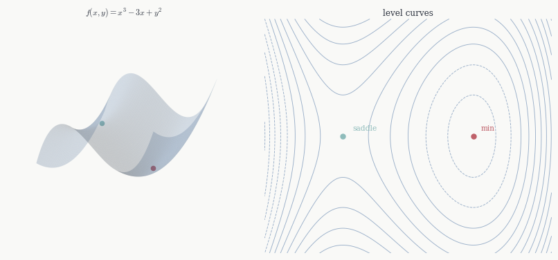
Example. Take f(x,y) = x^3 - 3x + y^2. The critical points come from \nabla f = (3x^2-3, 2y) = 0, giving (\pm 1, 0), and Hf(x,y) = \begin{pmatrix} 6x & 0 \\ 0 & 2 \end{pmatrix}. At (1,0): \det H = 12 > 0 and A = 6 > 0, so a local minimum with f(1,0) = -2. At (-1,0): \det H = -12 < 0, so a saddle. Notice that f has no global minimum on \mathbb{R}^2 — it goes to -\infty along the x-axis as x \to -\infty — so the local minimum at (1,0) is not a global one.

8.2 Global Extrema on Compact Sets

The second derivative test says nothing about global extrema — it is a purely local statement. For global questions we need the extreme value Theorem 2.4: a continuous function on a compact set attains its maximum and minimum. For a smooth function on an open set U, the domain is not compact and global extrema may not exist. But on a compact subset K \subset U they do, and the structure of critical points tells us where to look.

Any interior global extremum is also a local extremum, hence a critical point. So the global maximum and minimum on K are among the critical points of f in the interior of K, together with whatever happens on the boundary \partial K. The boundary is a lower-dimensional compact set, so the same argument applies recursively there — and when \partial K is a smooth submanifold, Lagrange multipliers give the critical points on it. The procedure is therefore: find all interior critical points, find all constrained critical points on \partial K, evaluate f at all of them, and take the largest and smallest values.

8.3 Constrained Optimisation

Now suppose we want to optimise f not over all of U but subject to a constraint: x must lie on a smooth submanifold M \subset U. The canonical case is a single equality constraint g(x) = c, where c is a regular value of g, so M = g^{-1}(c) is a smooth hypersurface.

The key is to think about what it means for a \in M to be a local extremum of f|_M. Take any smooth curve \gamma in M passing through a at t = 0. The composition f \circ \gamma : \mathbb{R} \to \mathbb{R} is an ordinary single-variable function, and if a is a local extremum of f|_M then f \circ \gamma has a critical point at t = 0, so (f \circ \gamma)'(0) = 0. By the chain rule this is Df_a(\gamma'(0)) = 0.

Now \gamma'(0) can be any tangent vector to M at a — by definition, T_aM is exactly the set of all such velocities. So the condition for a to be a constrained critical point is: Df_a(v) = 0 \quad \text{for every } v \in T_aM. In other words, Df_a must vanish on T_aM. Since M = g^{-1}(c) and c is a regular value, Chapter 2 tells us T_aM = \ker Dg_a. So Df_a vanishes on \ker Dg_a. But Dg_a \neq 0 (regularity), so \ker Dg_a is a hyperplane of dimension n-1. A linear functional that vanishes on a hyperplane is either the zero functional or a scalar multiple of the functional that defines that hyperplane. So either Df_a = 0 or Df_a = \lambda\, Dg_a for some \lambda \in \mathbb{R}. Either way the conclusion is Df_a = \lambda\, Dg_a.

Theorem 8.2 (Lagrange multiplier theorem) Let f, g \in C^1(U) and let c be a regular value of g. If a \in g^{-1}(c) is a local extremum of f|_{g^{-1}(c)}, then there exists \lambda \in \mathbb{R} such that \nabla f(a) = \lambda\, \nabla g(a).

Proof. As argued above, Df_a = \lambda\, Dg_a for some \lambda. Taking Riesz representatives on both sides gives \nabla f(a) = \lambda\, \nabla g(a). \square

The geometric picture is worth pausing on. The condition \nabla f(a) = \lambda\, \nabla g(a) says the two gradients are parallel, which means the level sets \{f = f(a)\} and \{g = c\} are tangent to each other at a. If instead the level sets of f crossed the constraint \{g = c\} at a, then f would be increasing on one side of the crossing and decreasing on the other — so you could increase f by moving along the constraint, contradicting the assumption that a is a maximum. The Lagrange condition is precisely the geometric statement that this crossing cannot happen.

Example. Minimise f(x,y) = x^2 + 2y^2 on the unit circle x^2+y^2=1.

We need \nabla f = \lambda \nabla g where g = x^2+y^2, i.e.
(2x, 4y) = \lambda(2x, 2y). From the first component, either x = 0 or \lambda = 1. From the second, either y = 0 or \lambda = 2.

If \lambda = 1: the second equation forces y = 0, and the constraint gives x = \pm 1 with f = 1.

If \lambda = 2: the first equation forces x = 0, and the constraint gives y = \pm 1 with f = 2.

Since the constraint circle is compact, f|_M attains both its maximum and minimum among these four candidates. The minimum is f = 1 at (\pm 1, 0) and the maximum is f = 2 at (0, \pm 1).

Multiple constraints. When M = F^{-1}(0) is cut out by k independent equations F = (g_1, \ldots, g_k), the tangent space is T_aM = \ker DF_a — the common kernel of the k functionals Dg_1|_a, \ldots, Dg_k|_a. The same argument gives: Df_a vanishes on this kernel, and a functional that vanishes on the intersection of k independent hyperplanes lies in their span. So

\nabla f(a) = \lambda_1 \nabla g_1(a) + \cdots + \lambda_k \nabla g_k(a)

with one multiplier per constraint. The rank condition for M to be a smooth submanifold — that the k functionals Dg_i|_a are linearly independent — is exactly what makes the span argument work.

Example. Minimise f(x,y,z) = x + 2y + 3z subject to g_1 = x^2+y^2+z^2 = 1 and g_2 = x+y+z = 0.

The condition (1,2,3) = 2\lambda_1(x,y,z) + \lambda_2(1,1,1) gives 1 = 2\lambda_1 x + \lambda_2, 2 = 2\lambda_1 y + \lambda_2, 3 = 2\lambda_1 z + \lambda_2. Subtracting consecutive equations: y - x = z - y = 1/(2\lambda_1), so x,y,z form an arithmetic sequence with common difference d. The constraint g_2 = 0 gives 3y = 0, so y = 0 and x = -d, z = d. The constraint g_1 = 1 gives 2d^2 = 1, so d = \pm 1/\sqrt{2}.

At d = 1/\sqrt{2}: f = -1/\sqrt{2} + 3/\sqrt{2} = \sqrt{2}. At d = -1/\sqrt{2}: f = -\sqrt{2}. The minimum is -\sqrt{2}.

8.4 A Remark on Sufficiency

The Lagrange condition is necessary for a constrained extremum, not sufficient. It identifies the candidates; it does not say which are maxima, minima, or saddle points on M.

When M is compact this is not a problem in practice. The extreme value theorem guarantees that f|_M attains its maximum and minimum, and both must occur at Lagrange points. So we compute all solutions to the Lagrange conditions, evaluate f at each, and compare — the largest value is the constrained maximum, the smallest is the constrained minimum. This is the procedure used in both examples above.

When M is not compact one has to argue separately that a maximum or minimum exists before applying this strategy. Often a geometric or physical argument does this: if f grows without bound along M as \|x\| \to \infty then a minimum must exist, and the Lagrange conditions find it. But existence cannot be taken for granted, and there are constrained optimisation problems where the Lagrange conditions have solutions but none of them are genuine extrema.