10 Multiple Integrals
Integration in one variable is conceptually clear: partition [a,b] into subintervals, approximate f on each by a constant, sum, and take the limit as the mesh goes to zero. In \mathbb{R}^n the same idea works with almost no modification — partition a box into sub-boxes, approximate f on each by a constant, sum. The definition is the same; only the geometry of the domain changes.
What is genuinely new in higher dimensions is the change of variables theorem. In one variable the substitution rule is \int_a^b f(g(t)) g'(t)\, dt = \int_{g(a)}^{g(b)} f(x)\, dx — a formula involving the derivative g'. In \mathbb{R}^n the correct generalisation replaces g' by |\det Dg|, the absolute value of the determinant of the Jacobian. The determinant measures how g scales volumes near each point, and the change of variables formula says the integral transforms exactly by this scaling factor. The inverse function theorem, proved in Chapter 7, is what makes the proof work.
We work with the Riemann integral throughout. For the theorems here — Fubini, change of variables, and improper integrals on reasonable domains — the Riemann framework is sufficient. Where it genuinely runs into trouble is with limits of integrals of non-uniform sequences of functions, or with domains so irregular that the boundary contributes to the integral. Handling these properly requires Lebesgue measure theory, which belongs in a different course. We note the places where the Riemann framework is being stretched and leave the full treatment there.
10.1 The Riemann Integral on a Box
A closed box in \mathbb{R}^n is a product of closed intervals: B = [a_1, b_1] \times \cdots \times [a_n, b_n]. A partition of B is a choice of partitions a_i = t_0^{(i)} < t_1^{(i)} < \cdots < t_{k_i}^{(i)} = b_i of each factor interval. This subdivides B into sub-boxes B_\alpha = [t_{\alpha_1-1}^{(1)}, t_{\alpha_1}^{(1)}] \times \cdots \times [t_{\alpha_n-1}^{(n)}, t_{\alpha_n}^{(n)}], indexed by multi-indices \alpha. The mesh of the partition is the largest side-length of any sub-box.
For a bounded function f : B \to \mathbb{R}, define the upper and lower Darboux sums: U(f, P) = \sum_\alpha M_\alpha\, \mathrm{vol}(B_\alpha), \qquad L(f, P) = \sum_\alpha m_\alpha\, \mathrm{vol}(B_\alpha), where M_\alpha = \sup_{B_\alpha} f, m_\alpha = \inf_{B_\alpha} f, and \mathrm{vol}(B_\alpha) = \prod_i (t_{\alpha_i}^{(i)} - t_{\alpha_i - 1}^{(i)}) is the volume of the sub-box.
Definition 10.1 (Riemann integrable) A bounded function f : B \to \mathbb{R} is Riemann integrable on B if \sup_P L(f, P) = \inf_P U(f, P), where the supremum and infimum are over all partitions P. The common value is the integral \int_B f, also written \int_B f(x)\, dx or \int_B f(x_1, \ldots, x_n)\, dx_1 \cdots dx_n.
The supremum of lower sums and infimum of upper sums always satisfy \sup_P L \leq \inf_P U — any lower sum is bounded above by any upper sum since m_\alpha \leq M_\alpha on each sub-box. Integrability asks that they actually meet.
Theorem 10.1 (Continuous functions are integrable) If f : B \to \mathbb{R} is continuous, it is Riemann integrable on B.
Proof. B is compact, so f is uniformly continuous: for every \varepsilon > 0 there exists \delta > 0 with |f(x) - f(y)| < \varepsilon / \mathrm{vol}(B) whenever \|x-y\| < \delta. Take any partition with mesh less than \delta\sqrt{n} — so any two points in the same sub-box are within \delta of each other. Then M_\alpha - m_\alpha < \varepsilon / \mathrm{vol}(B) on each sub-box, and U(f,P) - L(f,P) = \sum_\alpha (M_\alpha - m_\alpha)\,\mathrm{vol}(B_\alpha) < \frac{\varepsilon}{\mathrm{vol}(B)} \sum_\alpha \mathrm{vol}(B_\alpha) = \varepsilon. \qquad \square
More generally, a bounded function is Riemann integrable if and only if it is continuous except on a set of measure zero — a set that can be covered by boxes of arbitrarily small total volume. Functions with finitely many discontinuities, or discontinuities along a smooth curve, are integrable. This characterisation uses the language of Lebesgue measure; we state it as a fact and note that all functions we integrate in practice satisfy it.
The integral is linear: \int_B (\alpha f + \beta g) = \alpha \int_B f + \beta \int_B g. It is monotone: f \leq g implies \int_B f \leq \int_B g. And it satisfies |\int_B f| \leq \int_B |f| \leq \|f\|_\infty\,\mathrm{vol}(B). All of these follow from the corresponding inequalities for Darboux sums.
10.2 Integration on Bounded Domains
Most domains of interest are not boxes. To integrate over a bounded open set \Omega \subset \mathbb{R}^n, the natural approach is to enclose \Omega in a box B and extend f to be zero outside \Omega.
Definition 10.2 (Integral over a bounded domain) Let \Omega \subset \mathbb{R}^n be bounded and f : \Omega \to \mathbb{R} bounded. Enclose \Omega in a box B and define \tilde{f}(x) = \begin{cases} f(x) & x \in \Omega \\ 0 & x \notin \Omega. \end{cases} If \tilde{f} is Riemann integrable on B, we say f is integrable on \Omega and define \int_\Omega f = \int_B \tilde{f}. The result is independent of the choice of B.
The issue with this approach is the boundary \partial\Omega. The function \tilde{f} is discontinuous at every boundary point where f \neq 0, so integrability of \tilde{f} requires that \partial\Omega have measure zero. Domains with smooth boundaries — balls, regions bounded by smooth surfaces, images of smooth maps — have this property. Domains with fractal boundaries may not. We restrict attention to domains with smooth or piecewise-smooth boundaries and treat the Riemann framework as adequate.
10.3 Fubini’s Theorem
The practical value of the multivariable integral comes from the ability to compute it as a sequence of one-variable integrals. This is Fubini’s theorem.
Theorem 10.2 (Fubini’s theorem) Let f : B \to \mathbb{R} be continuous on the box B = B' \times B'' where B' \subset \mathbb{R}^k and B'' \subset \mathbb{R}^{n-k}. Then \int_B f(x', x'')\, d(x',x'') = \int_{B'} \left(\int_{B''} f(x', x'')\, dx''\right) dx' = \int_{B''} \left(\int_{B'} f(x', x'')\, dx'\right) dx''.
In words: to integrate over a box, integrate first over the second factor (treating x' as fixed to get a function of x' alone), then integrate the result over the first factor. The order of integration does not matter.
The proof in full generality belongs with Lebesgue integration — the Riemann proof requires additional hypotheses to handle the case where the inner integral might not be Riemann integrable as a function of x' for every x''. For continuous f on a box this issue disappears: the inner integral g(x') = \int_{B''} f(x', x'')\, dx'' is continuous in x' by the dominated convergence theorem (which holds here by uniform continuity), so the outer integral is well-defined. The equality of the two iterated integrals follows by checking it for step functions — where both sides equal the same Darboux sum — and approximating f uniformly.
What Fubini really says is that the order of integration is irrelevant, and in practice it means we can compute \int_B f by iterating n one-variable integrals in any order we like.
Example. \int_0^1 \int_0^1 xe^{xy}\, dy\, dx. Integrating over y first: \int_0^1 xe^{xy}\, dy = [e^{xy}]_0^1 = e^x - 1. Then \int_0^1 (e^x - 1)\, dx = [e^x - x]_0^1 = (e-1) - 1 = e - 2.
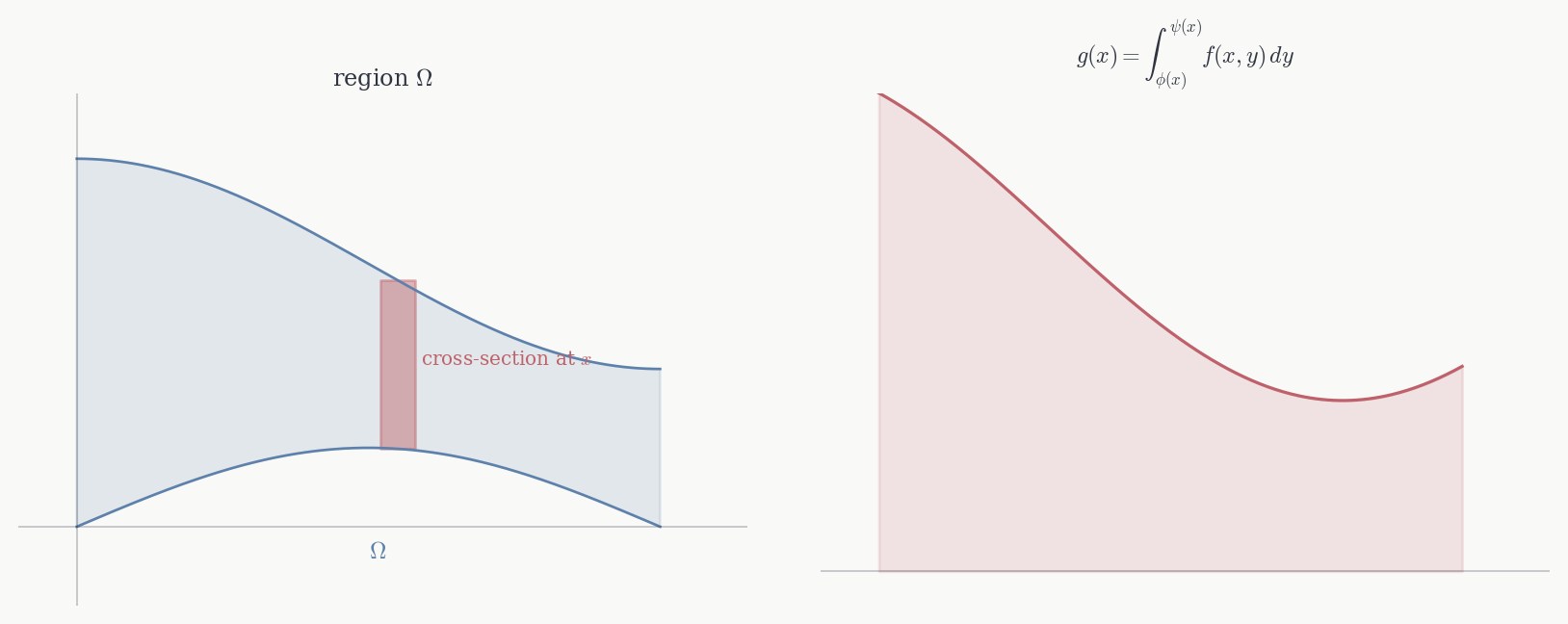
Fubini extends to non-rectangular domains by the standard stratification: for a region \Omega = \{(x,y) : a \leq x \leq b,\; \phi(x) \leq y \leq \psi(x)\} with \phi, \psi continuous, \int_\Omega f = \int_a^b \int_{\phi(x)}^{\psi(x)} f(x,y)\, dy\, dx. The inner integral is over the cross-section of \Omega at height x, and the outer integral sweeps over all x.
10.4 The Change of Variables Theorem
The most important computational tool for multivariable integrals is the change of variables theorem. It says: if g : \Omega \to g(\Omega) is a diffeomorphism, then \int_{g(\Omega)} f(y)\, dy = \int_\Omega f(g(x))\, |\det Dg_x|\, dx. The factor |\det Dg_x| is the absolute value of the Jacobian determinant of g at x. It measures the local volume scaling of g: if g stretches volume by a factor of |\det Dg_x| near x, then the integral scales by exactly that factor. This is the precise multivariable generalisation of the one-variable substitution rule \int f(g(t)) g'(t)\, dt = \int f(y)\, dy.
Theorem 10.3 (Change of variables) Let \Omega \subset \mathbb{R}^n be a bounded open set and g : \Omega \to \mathbb{R}^n a C^1 injective map with |\det Dg_x| > 0 on \Omega. Let f : g(\Omega) \to \mathbb{R} be continuous. Then \int_{g(\Omega)} f(y)\, dy = \int_\Omega f(g(x))\,|\det Dg_x|\, dx.
Before the proof, the factor |\det Dg_x| deserves some motivation. The determinant of a linear map T measures the signed volume of the image of the unit cube under T. Near a point x, the map g is approximately linear — it looks like Dg_x — so it scales the volume of a small box near x by approximately |\det Dg_x|. Summing these local scalings over the domain \Omega gives the global volume scaling, and the integral transforms accordingly.
To make this precise, we need to know how |\det Dg| behaves under composition, and what it means for the image of a box under a linear map. Two facts from linear algebra are central: first, \det(AB) = \det(A)\det(B) — the determinant is multiplicative; second, a linear map T sends a box of volume V to a region of volume |\det T| \cdot V — the absolute determinant is the volume scaling factor.
Proof. We prove the result in three steps of increasing generality.
Step 1: linear maps. If g = T is a linear map and \Omega = [0,1]^n, then g(\Omega) = T([0,1]^n) has volume |\det T|, and the formula reads \int_{T([0,1]^n)} f\, dy = \int_{[0,1]^n} f(Tx)\, |\det T|\, dx. For f = 1 this is just the volume formula. For general f it follows by approximating f by step functions and using linearity of the integral.
Step 2: maps that are close to the identity. Suppose g : B \to \mathbb{R}^n is a diffeomorphism on a box B with g(x) = x + \phi(x) where \phi is small in C^1. Partition B into small sub-boxes B_\alpha. On each B_\alpha, the map g is approximately the affine map x \mapsto g(x_\alpha) + Dg_{x_\alpha}(x - x_\alpha) where x_\alpha is the centre. By Step 1, this affine map sends B_\alpha to a region of volume approximately |\det Dg_{x_\alpha}| \cdot \mathrm{vol}(B_\alpha). Summing over sub-boxes and taking the partition mesh to zero gives the formula in this case, using the fact that |\det Dg_x| is uniformly continuous on the compact closure of B.
Step 3: general diffeomorphisms. By the inverse function theorem, every C^1 diffeomorphism g : \Omega \to g(\Omega) can be written locally as a composition of maps, each of which changes only one coordinate at a time (this uses the fact that any invertible matrix is a product of elementary matrices). For a map that changes only the k-th coordinate, the formula reduces to a one-variable substitution applied to the k-th integral in a Fubini iteration. Composing these gives the general case, with determinant factors multiplying by the chain rule \det D(g_2 \circ g_1) = (\det Dg_2) \circ g_1 \cdot \det Dg_1. \square
The proof as written is a sketch — turning Step 2 into a rigorous estimate and Step 3 into a precise decomposition requires careful bookkeeping that we suppress. The key ideas are all there: local approximation by linear maps, determinant as volume scaling, and the chain rule for determinants.
Example: polar coordinates. Let g(r,\theta) = (r\cos\theta, r\sin\theta) on \Omega = (0,\infty) \times (0, 2\pi). Then \det Dg_{(r,\theta)} = r, and the theorem gives \int_{g(\Omega)} f(x,y)\, dx\, dy = \int_0^\infty \int_0^{2\pi} f(r\cos\theta, r\sin\theta)\, r\, dr\, d\theta. The factor r is the Jacobian factor. For f = 1 this correctly gives the area of \mathbb{R}^2 \setminus \{0\} as \int_0^\infty \int_0^{2\pi} r\, d\theta\, dr — divergent, as expected since the plane has infinite area. For f(x,y) = e^{-(x^2+y^2)}: \int_{\mathbb{R}^2} e^{-(x^2+y^2)}\, dx\, dy = \int_0^\infty e^{-r^2} r \left(\int_0^{2\pi} d\theta\right) dr = 2\pi \int_0^\infty r e^{-r^2}\, dr = \pi. Since the double integral factors as \left(\int_{-\infty}^\infty e^{-x^2} dx\right)^2, this gives \int_{-\infty}^\infty e^{-x^2}\, dx = \sqrt{\pi} — the Gaussian integral, recovered by polar coordinates.
Example: spherical coordinates. The map g(r,\phi,\theta) = (r\sin\phi \cos\theta, r\sin\phi\sin\theta, r\cos\phi) on (0,\infty) \times (0,\pi) \times (0, 2\pi) has |\det Dg| = r^2\sin\phi, giving \int_{\mathbb{R}^3} f\, dx\, dy\, dz = \int_0^\infty\int_0^\pi\int_0^{2\pi} f(g(r,\phi,\theta))\, r^2\sin\phi\, d\theta\, d\phi\, dr.
10.5 Improper Integrals
The Riemann integral as defined requires f to be bounded and \Omega to be bounded. Many natural integrals violate one or both conditions — the Gaussian integral above integrated over all of \mathbb{R}^2, volumes of unbounded regions, integrals of functions with singularities. We handle these by exhaustion.
Definition 10.3 (Improper integral) Let \Omega \subset \mathbb{R}^n be open (possibly unbounded) and f : \Omega \to \mathbb{R} continuous (possibly unbounded near \partial\Omega). Suppose \Omega_1 \subset \Omega_2 \subset \cdots is an increasing sequence of bounded open sets with compact closures in \Omega and \bigcup_k \Omega_k = \Omega. If f is integrable on each \Omega_k and \lim_{k \to \infty} \int_{\Omega_k} |f| exists and is finite, we say f is improperly integrable on \Omega and define \int_\Omega f = \lim_{k\to\infty} \int_{\Omega_k} f.
The condition on |f| rather than f is the right one — it ensures the integral is absolutely convergent, meaning it does not depend on the choice of exhaustion sequence (\Omega_k) or on the order in which we accumulate the domain. An integral that converges but not absolutely — where the positive and negative parts both diverge but cancel — is much harder to work with in higher dimensions, because there is no canonical order in which to accumulate \mathbb{R}^n the way there is on the real line.
Example. The integral \int_{\mathbb{R}^n} e^{-\|x\|^2}\, dx converges: take \Omega_k = B(0,k) and use polar or spherical coordinates. We computed \int_{\mathbb{R}^2} e^{-\|x\|^2} = \pi above; more generally \int_{\mathbb{R}^n} e^{-\|x\|^2} = \pi^{n/2}.
Example. The integral \int_{\mathbb{R}^2} \frac{1}{1 + \|x\|^2}\, dx diverges: in polar coordinates the integral over B(0,R) is \int_0^R \int_0^{2\pi} \frac{r}{1+r^2}\, d\theta\, dr = \pi \ln(1+R^2) \to \infty.
Near singularities. For an integrand with a singularity at 0, take \Omega_k = \{x : 1/k < \|x\| < k\} as the exhaustion. For example, \int_{B(0,1)} \|x\|^{-\alpha}\, dx converges in \mathbb{R}^n if and only if \alpha < n: in spherical coordinates it becomes C\int_0^1 r^{-\alpha} r^{n-1}\, dr = C\int_0^1 r^{n-1-\alpha}\, dr, which converges iff n - 1 - \alpha > -1, i.e. \alpha < n.
The change of variables theorem extends to improper integrals by applying it on each \Omega_k and passing to the limit, provided the Jacobian factor |\det Dg| is bounded away from zero on compact subsets of \Omega.
10.6 A Remark on Measure Theory
The Riemann integral handles everything needed for this course. But it has genuine limitations. It cannot integrate the characteristic function of the rationals (which equals 1 on \mathbb{Q} and 0 elsewhere) — the upper sum is always 1 and the lower sum always 0. More practically, it behaves badly under pointwise limits: if f_k \to f pointwise, \int f_k need not converge to \int f without uniform convergence, which is often hard to verify. The dominated convergence theorem — which says pointwise convergence plus a uniform bound implies convergence of integrals — is a Lebesgue result that has no clean Riemann analogue.
Lebesgue integration assigns a measure to sets (capturing “how large” they are) and defines the integral via this measure. The resulting theory is strictly more powerful: every Riemann integrable function is Lebesgue integrable with the same value, the dominated convergence theorem holds, and L^p spaces of functions with \int |f|^p < \infty are complete — a fact that underlies Fourier analysis, functional analysis, and the rigorous theory of probability. For the integral theorems of the next part and for integration on surfaces, the Riemann framework suffices and we stay within it. But the reader should know the boundary they are working near.